Probability and Statistics

Est. read time: 5 minutes | Last updated: July 17, 2026 by John Gentile

Contents

Distributions
- Gaussian Random Variable
Detection Theory
Estimation Theory
- Maximum Likelihood Estimation
  - Example: MLE for the Gaussian Mean
Covariance Matrices
References

import numpy as np
import matplotlib.pyplot as plt

from sympy import *
init_printing()

Distributions

There are several distributions relevant to detection and estimation. The Probability Density Function (PDF) $f(x)$ gives the probability that a random vairable will take the value $x$ .

The main central moments are:

Mean/Expectation: $\mu = E[X]$
Variance: $\sigma^{2} = E \left[ (X - \mu)^{2} \right]$

Where $E \{ \cdot \}$ is the expectation operator:

E\{g(x)\} = \int_{-\infty}^{\infty} g(x)f(x)dx

Other notations:

The operator $\sim$ means “is distributed as”.
$f_{X}(x)$ means the distribution $X$ is used in the PDF.

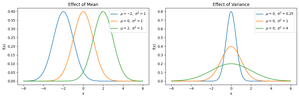
Gaussian Random Variable

The Gaussian, or normal, distribution is defined with mean and variance of:

$E [x] = \mu$
$E \left[ (x - \mu)^{2} \right] = \sigma^{2}$

It is parameterized as:

X \sim \mathcal{N}\left( \mu,\sigma^{2} \right)

With PDF implemented as:

f_{\mathcal{N}}(x|\mu,\sigma) = \frac{1}{\sigma\sqrt{2\pi}}e^{-\frac{(x-\mu)^{2}}{2\sigma^{2}}}

def normal_pdf(x: np.ndarray, mu: float, sigma: float) -> np.ndarray:
    return (1 / (sigma * np.sqrt(2 * np.pi))) * np.exp(-0.5 * ((x - mu) / sigma) ** 2)

samples = np.linspace(-6, 6, 500)
fig, axes = plt.subplots(1, 2, figsize=(12, 4))

# Vary mean with fixed variance
for mu in [-2, 0, 2]:
    sigma = 1
    axes[0].plot(samples, normal_pdf(samples, mu, sigma), label=rf"$\mu={mu},\ \sigma^2={sigma**2}$")
axes[0].set_title("Effect of Mean")
axes[0].set_xlabel("x")
axes[0].set_ylabel("f(x)")
axes[0].legend()

# Vary variance with fixed mean
for sigma in [0.5, 1, 2]:
    mu = 0
    axes[1].plot(samples, normal_pdf(samples, mu, sigma), label=rf"$\mu={mu},\ \sigma^2={sigma**2}$")
axes[1].set_title("Effect of Variance")
axes[1].set_xlabel("x")
axes[1].set_ylabel("f(x)")
axes[1].legend()

plt.tight_layout()
plt.show()

png

Detection Theory

Usually called hypothesis testing, in DSP the simplest form of signal detection is shown as a binary hypothesis- the two hypotheses are commonly referred to as the null hypothesis ( $H_{0}$ , signal is absent) and the alternative hypothesis ( $H_{1}$ , signal is present)

Estimation Theory

Maximum Likelihood Estimation

Maximum Likelihood Estimation (MLE) is a method for estimating the parameters of a distribution given observed data. The idea is to choose the parameters that make the observed data most probable.

Given $N$ independent observations $x_1, x_2, \ldots, x_N$ drawn from a distribution with parameter(s) $\theta$ , the likelihood function is the joint probability of the data:

L(\theta) = \prod_{i=1}^{N} f(x_i \mid \theta)

In practice we work with the log-likelihood (since products become sums):

\ell(\theta) = \ln L(\theta) = \sum_{i=1}^{N} \ln f(x_i \mid \theta)

The MLE is the value $\hat{\theta}$ that maximizes $\ell(\theta)$ :

\hat{\theta} = \arg\max_{\theta} \; \ell(\theta)

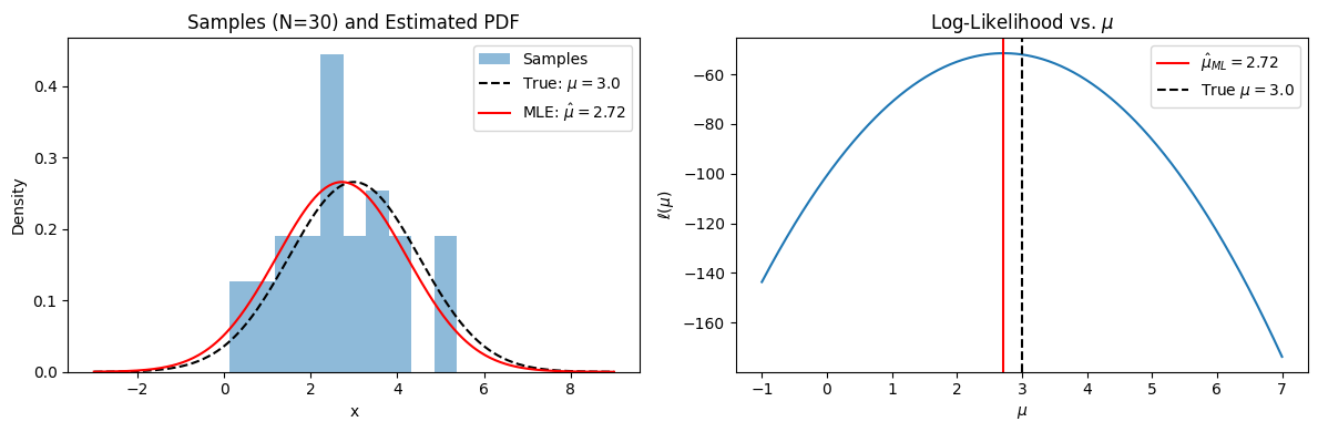
Example: MLE for the Gaussian Mean

If we assume $x_i \sim \mathcal{N}(\mu, \sigma^2)$ with known $\sigma^2$ , the log-likelihood as a function of $\mu$ is:

\ell(\mu) = -\frac{N}{2}\ln(2\pi\sigma^2) - \frac{1}{2\sigma^2}\sum_{i=1}^{N}(x_i - \mu)^2

Setting $\frac{d\ell}{d\mu} = 0$ and solving gives the familiar result:

\hat{\mu}_{ML} = \frac{1}{N}\sum_{i=1}^{N} x_i = \bar{x}

The MLE of the mean is simply the sample mean.

np.random.seed(42)

# Generate samples from a known Gaussian
true_mu = 3.0
true_sigma = 1.5
N = 30
samples = np.random.normal(true_mu, true_sigma, N)

# Compute log-likelihood over a range of candidate mu values (sigma known)
mu_range = np.linspace(-1, 7, 500)
log_likelihood = np.array([
    -N/2 * np.log(2 * np.pi * true_sigma**2)
    - 1/(2 * true_sigma**2) * np.sum((samples - mu)**2)
    for mu in mu_range
])

mu_ml = np.mean(samples)

fig, (ax1, ax2) = plt.subplots(1, 2, figsize=(12, 4))

# Left: the observed samples and the true vs estimated distributions
ax1.hist(samples, bins=10, density=True, alpha=0.5, label="Samples")
x_plot = np.linspace(-3, 9, 300)
ax1.plot(x_plot,
         (1 / (true_sigma * np.sqrt(2 * np.pi))) * np.exp(-0.5 * ((x_plot - true_mu) / true_sigma)**2),
         "k--", label=rf"True: $\mu={true_mu}$")
ax1.plot(x_plot,
         (1 / (true_sigma * np.sqrt(2 * np.pi))) * np.exp(-0.5 * ((x_plot - mu_ml) / true_sigma)**2),
         "r-", label=rf"MLE: $\hat={mu_ml:.2f}$")
ax1.set_xlabel("x")
ax1.set_ylabel("Density")
ax1.set_title(f"Samples (N={N}) and Estimated PDF")
ax1.legend()

# Right: the log-likelihood curve
ax2.plot(mu_range, log_likelihood)
ax2.axvline(mu_ml, color="r", linestyle="-", label=rf"$\hat_={mu_ml:.2f}$")
ax2.axvline(true_mu, color="k", linestyle="--", label=rf"True $\mu={true_mu}$")
ax2.set_xlabel(r"$\mu$")
ax2.set_ylabel(r"$\ell(\mu)$")
ax2.set_title(r"Log-Likelihood vs. $\mu$")
ax2.legend()

plt.tight_layout()
plt.show()

png

Covariance Matrices

For a random vector $\mathbf{x} = [x_1, x_2, \ldots, x_M]^T$ with mean $\boldsymbol{\mu} = E\{\mathbf{x}\}$ , the covariance matrix is:

\mathbf{R}_{xx} = E\left\{ (\mathbf{x} - \boldsymbol{\mu})(\mathbf{x} - \boldsymbol{\mu})^H \right\}

where $(\cdot)^H$ denotes the conjugate transpose (Hermitian conjugate). Each element $(i,j)$ of $\mathbf{R}_{xx}$ is the covariance between $x_i$ and $x_j$ :

R_{ij} = E\{(x_i - \mu_i)(x_j - \mu_j)^*\}

The diagonal entries are the variances $\sigma_i^2$ of each element.

Key Properties

Hermitian: $\mathbf{R}_{xx} = \mathbf{R}_{xx}^H$ (symmetric for real data)
Positive semi-definite: $\mathbf{a}^H \mathbf{R}_{xx} \mathbf{a} \geq 0$ for all $\mathbf{a}$ , meaning all eigenvalues $\lambda_i \geq 0$
Eigendecomposition: $\mathbf{R}_{xx} = \mathbf{U} \boldsymbol{\Lambda} \mathbf{U}^H$ where $\mathbf{U}$ is unitary and $\boldsymbol{\Lambda} = \text{diag}(\lambda_1, \ldots, \lambda_M)$

Sample Covariance Matrix

In practice we estimate $\mathbf{R}_{xx}$ from $N$ observation snapshots $\mathbf{x}_1, \ldots, \mathbf{x}_N$ :

\hat{\mathbf{R}}_{xx} = \frac{1}{N} \sum_{n=1}^{N} \mathbf{x}_n \mathbf{x}_n^H

(assuming zero-mean data, or after subtracting the sample mean). As $N \to \infty$ , $\hat{\mathbf{R}} \to \mathbf{R}$ .

Relevance to Array Processing

Covariance matrices are key in array signal processing; in sensor array processing (e.g. radar, sonar, communications), $\mathbf{x}$ is the snapshot vector across $M$ antenna elements. The covariance matrix encodes the spatial structure of all impinging signals and noise. Algorithms like MVDR beamforming and MUSIC operate directly on $\mathbf{R}_{xx}$ (or its estimate) to detect signals and estimate their directions of arrival.

Snapshot Support: How Many Snapshots Are Enough?

A central practical question is how many snapshots we need to estimate $\mathbf{R}$ well enough. Too few gives a noisy, ill-conditioned estimate; too many forces the scene (source angles, interference powers) to stay stationary over a long collection window — often unrealistic for moving platforms or agile emitters. So there is a sweet spot, and in practice the snapshot count $K$ for adaptive beamformers is often quoted in the rough range of 64–256 (this $K$ is the same snapshot count denoted $N$ in the estimator above).

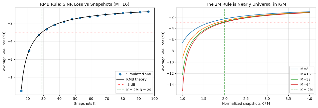
This range is not arbitrary. For an adaptive beamformer formed by inverting the sample covariance matrix — the Sample Matrix Inversion (SMI) method — the classic result is the Reed–Mallett–Brennan (RMB) rule (1974). If the array has $M$ degrees of freedom (here, $M$ elements) and the training snapshots contain interference + noise only, the average output SINR relative to the optimal known- $\mathbf{R}$ beamformer is:

E\{\rho\} = \frac{K - M + 2}{K + 1}, \qquad \rho = \frac{\text{SINR}_{\text{achieved}}}{\text{SINR}_{\text{optimal}}} \le 1

Setting $E\{\rho\} = \tfrac{1}{2}$ (a 3 dB SINR loss) and solving gives the famous rule of thumb — use roughly twice as many snapshots as array elements:

K \approx 2M \quad (\text{exactly 3 dB loss at } K = 2M - 3)

For arrays of 32–128 elements this is precisely the “64–256 snapshots” range seen in practice. Remarkably, the requirement is distribution-free in the scene: it depends only on the number of degrees of freedom $M$ , not on the interference powers or angles. The simulation below confirms the theoretical curve and shows that the curves for different $M$ collapse onto one another when plotted against the normalized snapshot count $K/M$ .

np.random.seed(1)

def steering_vector(theta_deg, M, d_lambda=0.5):
    """ULA steering vector: a_m(theta) = exp(j*2*pi*d*m*sin(theta))."""
    m = np.arange(M)
    return np.exp(1j * 2 * np.pi * d_lambda * m * np.sin(np.deg2rad(theta_deg)))

def interference_snapshots(A_i, powers, noise_power, K):
    """K snapshots of interference + noise only (the adaptive training data)."""
    J, M = A_i.shape[1], A_i.shape[0]
    S = np.sqrt(powers / 2)[:, None] * (np.random.randn(J, K) + 1j * np.random.randn(J, K))
    noise = np.sqrt(noise_power / 2) * (np.random.randn(M, K) + 1j * np.random.randn(M, K))
    return A_i @ S + noise

# --- Scenario: desired signal at boresight, 3 strong interferers, white noise ---
M = 16                                               # array elements = degrees of freedom
desired_angle = 0.0
interferer_angles = np.array([-40.0, -15.0, 25.0])
interferer_powers = np.array([100.0, 100.0, 100.0])  # 20 dB interference-to-noise ratio
noise_power = 1.0

a_d = steering_vector(desired_angle, M)
A_i = np.column_stack([steering_vector(t, M) for t in interferer_angles])

# True interference-plus-noise covariance and the optimal (clairvoyant) SINR
R_in = (A_i * interferer_powers) @ A_i.conj().T + noise_power * np.eye(M)
R_in_inv = np.linalg.inv(R_in)
sinr_opt = np.real(a_d.conj() @ R_in_inv @ a_d)      # desired signal power = 1

def sinr_loss(w):
    """Output SINR of weight vector w relative to optimal (scale-invariant, <= 1)."""
    achieved = np.abs(w.conj() @ a_d) ** 2 / np.real(w.conj() @ R_in @ w)
    return achieved / sinr_opt

# --- Monte Carlo: average SINR loss of the SMI beamformer vs number of snapshots ---
K_values = np.unique(np.round(np.linspace(M, 6 * M, 16)).astype(int))
n_trials = 500
rho_sim = []
for K in K_values:
    acc = 0.0
    for _ in range(n_trials):
        X = interference_snapshots(A_i, interferer_powers, noise_power, K)
        R_hat = (X @ X.conj().T) / K
        w_smi = np.linalg.solve(R_hat, a_d)          # SMI weights (proportional to R^-1 a_d)
        acc += sinr_loss(w_smi)
    rho_sim.append(acc / n_trials)
rho_sim = np.array(rho_sim)

# RMB theoretical mean loss: E[rho] = (K - M + 2) / (K + 1)
rmb = lambda K, M: (K - M + 2) / (K + 1)

fig, (ax1, ax2) = plt.subplots(1, 2, figsize=(13, 4.5))

# Left: simulation vs RMB theory for this M-element array
ax1.plot(K_values, 10 * np.log10(rho_sim), "o", label="Simulated SMI")
K_fine = np.arange(M, 6 * M + 1)
ax1.plot(K_fine, 10 * np.log10(rmb(K_fine, M)), "k-", label="RMB theory")
ax1.axhline(-3, color="r", ls=":", label="-3 dB")
ax1.axvline(2 * M - 3, color="g", ls="--", label=f"K = 2M-3 = {2 * M - 3}")
ax1.set_xlabel("Snapshots K")
ax1.set_ylabel("Average SINR loss (dB)")
ax1.set_title(f"RMB Rule: SINR Loss vs Snapshots (M={M})")
ax1.legend()
ax1.grid(alpha=0.3)

# Right: curves for several M collapse together when plotted against K/M
for M_p in [8, 16, 32, 64]:
    ratio = np.linspace(1, 4, 200)
    ax2.plot(ratio, 10 * np.log10(rmb(ratio * M_p, M_p)), label=f"M={M_p}")
ax2.axhline(-3, color="r", ls=":")
ax2.axvline(2, color="g", ls="--", label="K = 2M")
ax2.set_xlabel("Normalized snapshots K / M")
ax2.set_ylabel("Average SINR loss (dB)")
ax2.set_title("The 2M Rule is Nearly Universal in K/M")
ax2.legend()
ax2.grid(alpha=0.3)

plt.tight_layout()
plt.show()

png

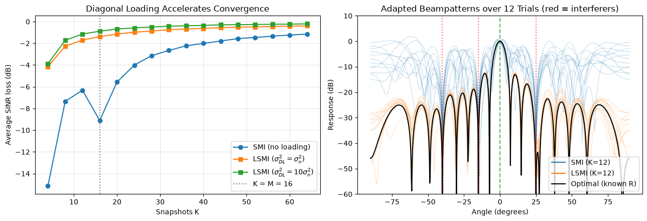
Diagonal Loading

The RMB rule assumes we invert the raw sample matrix $\hat{\mathbf{R}}$ . When snapshots are scarce ( $K \lesssim M$ ) this estimate is poorly conditioned — and for $K < M$ it is outright singular — so its inverse explosively amplifies estimation errors, producing noisy weights, high sidelobes, and self-nulling of the desired signal.

Diagonal loading regularizes the estimate by adding a scaled identity before inversion:

\hat{\mathbf{R}}_{\text{DL}} = \hat{\mathbf{R}} + \sigma_{\text{DL}}^2 \mathbf{I}

Because $\mathbf{I}$ shares its eigenvectors with every matrix, loading simply shifts all eigenvalues up by $\sigma_{\text{DL}}^2$ (i.e. $\lambda_i \to \lambda_i + \sigma_{\text{DL}}^2$ ) while leaving the eigenvectors untouched. This lifts the small, error-dominated noise-subspace eigenvalues away from zero, bounding the condition number and taming $\hat{\mathbf{R}}^{-1}$ . The resulting beamformer — Loaded SMI (LSMI) — has several equivalent interpretations:

Regularization: identical in form to Tikhonov regularization / ridge regression of the inverse.
Robust beamforming: equivalent to a worst-case design that protects against steering-vector mismatch within an uncertainty ball, whose radius sets the loading level.
Faster convergence: LSMI’s convergence depends on the number of dominant (interference) eigenvalues above the loading level — not the full dimension $M$ . With only a few strong interferers, LSMI reaches near-optimal SINR with far fewer than $2M$ snapshots, directly accelerating adaptation.

Choosing the loading level. A common rule of thumb places $\sigma_{\text{DL}}^2$ a few dB above the noise floor, typically $\sigma_{\text{DL}}^2 \approx (1\text{–}10)\,\sigma_n^2$ . Too little fails to regularize; too much biases the weights toward the non-adaptive (quiescent) beamformer and stops nulling interference.

Caveat for DoA estimation. Loading is excellent for beamforming, but for high-resolution spectral direction-of-arrival estimators (e.g. the Capon/MVDR spectrum) heavy loading broadens peaks and raises the spectral noise floor, which can bury weak sources. When the goal is angle estimation rather than output SINR, use light loading or none.

The experiment below contrasts plain SMI against LSMI: LSMI converges with dramatically fewer snapshots, and its adapted beampatterns stay stable (nulls on the interferers, unit gain on the desired angle) where SMI is erratic.

np.random.seed(2)

# --- SINR convergence: plain SMI vs Loaded SMI (LSMI) at two loading levels ---
K_values_dl = np.unique(np.round(np.linspace(4, 4 * M, 16)).astype(int))
loadings = {r"LSMI ($\sigma_{DL}^2 = \sigma_n^2$)": 1.0 * noise_power,
            r"LSMI ($\sigma_{DL}^2 = 10\sigma_n^2$)": 10.0 * noise_power}
n_trials = 500

rho_smi = []
rho_lsmi = {name: [] for name in loadings}
for K in K_values_dl:
    acc_smi = 0.0
    acc_l = {name: 0.0 for name in loadings}
    for _ in range(n_trials):
        X = interference_snapshots(A_i, interferer_powers, noise_power, K)
        R_hat = (X @ X.conj().T) / K
        # Plain SMI: pseudo-inverse stands in where R_hat is singular (K < M)
        acc_smi += sinr_loss(np.linalg.pinv(R_hat) @ a_d)
        for name, delta in loadings.items():
            acc_l[name] += sinr_loss(np.linalg.solve(R_hat + delta * np.eye(M), a_d))
    rho_smi.append(acc_smi / n_trials)
    for name in loadings:
        rho_lsmi[name].append(acc_l[name] / n_trials)

# --- Representative adapted beampatterns at a small snapshot count (K < M) ---
K_bp = 12
n_bp_trials = 12
theta = np.linspace(-90, 90, 721)
A_scan = np.column_stack([steering_vector(t, M) for t in theta])

def beampattern_db(w):
    w = w / (w.conj() @ a_d)                          # unit response at desired angle
    return 20 * np.log10(np.abs(w.conj() @ A_scan) + 1e-12)

w_opt = R_in_inv @ a_d                                # clairvoyant optimum

fig, (ax1, ax2) = plt.subplots(1, 2, figsize=(13, 4.5))

# Left: average SINR loss vs snapshots, SMI vs LSMI
ax1.plot(K_values_dl, 10 * np.log10(rho_smi), "o-", label="SMI (no loading)")
for name in loadings:
    ax1.plot(K_values_dl, 10 * np.log10(rho_lsmi[name]), "s-", label=name)
ax1.axvline(M, color="gray", ls=":", label=f"K = M = {M}")
ax1.set_xlabel("Snapshots K")
ax1.set_ylabel("Average SINR loss (dB)")
ax1.set_title("Diagonal Loading Accelerates Convergence")
ax1.legend()
ax1.grid(alpha=0.3)

# Right: overlaid beampatterns over several trials at K < M
for _ in range(n_bp_trials):
    X = interference_snapshots(A_i, interferer_powers, noise_power, K_bp)
    R_hat = (X @ X.conj().T) / K_bp
    ax2.plot(theta, beampattern_db(np.linalg.pinv(R_hat) @ a_d), color="C0", alpha=0.25, lw=0.8)
    ax2.plot(theta, beampattern_db(np.linalg.solve(R_hat + 10 * noise_power * np.eye(M), a_d)),
             color="C1", alpha=0.25, lw=0.8)
ax2.plot([], [], color="C0", label=f"SMI (K={K_bp})")
ax2.plot([], [], color="C1", label=f"LSMI (K={K_bp})")
ax2.plot(theta, beampattern_db(w_opt), "k-", lw=1.5, label="Optimal (known R)")
for t in interferer_angles:
    ax2.axvline(t, color="r", ls=":", alpha=0.6)
ax2.axvline(desired_angle, color="g", ls="--", alpha=0.6)
ax2.set_ylim(-60, 10)
ax2.set_xlabel("Angle (degrees)")
ax2.set_ylabel("Response (dB)")
ax2.set_title(f"Adapted Beampatterns over {n_bp_trials} Trials (red = interferers)")
ax2.legend(loc="lower right")

plt.tight_layout()
plt.show()

png

References

Think Stats, 3rd Edition - Allen Downey
Introduction to Modern Statistics
Probability, Statistics and Random Processes - Free Course
H. L. Van Trees, Optimum Array Processing (Detection, Estimation, and Modulation Theory, Part IV), Wiley, 2002.
I. S. Reed, J. D. Mallett, and L. E. Brennan, “Rapid Convergence Rate in Adaptive Arrays,” IEEE Transactions on Aerospace and Electronic Systems, vol. AES-10, no. 6, 1974 — the RMB ( $K \approx 2M$ ) rule.
B. D. Carlson, “Covariance Matrix Estimation Errors and Diagonal Loading in Adaptive Arrays,” IEEE Transactions on Aerospace and Electronic Systems, vol. 24, no. 4, 1988 — diagonal loading / Loaded SMI.