Emitter Geolocation

Est. read time: 1 minute | Last updated: June 16, 2026 by John Gentile

Contents

References

import numpy as np
import matplotlib.pyplot as plt

from rfproto import impairments, plot, sig_gen

import plotly.graph_objects as go
import plotly.io as pio
pio.renderers.default = "png" # "notebook_connected" 

fs = 10e6
num_chirp_samples = 2000
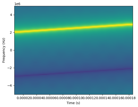
upchirp = sig_gen.cmplx_dt_lfm_chirp(2.0, 2e6, 3e6, fs, num_chirp_samples)
plt.specgram(upchirp, pad_to=1024, Fs=fs)
plt.xlabel('Time (s)')
plt.ylabel('Frequency (Hz)')
plt.show()

png

pulse_plus_noise = impairments.awgn(1.0, 5 * num_chirp_samples)
pulse_plus_noise[3000:5000] += upchirp
plt.specgram(pulse_plus_noise, pad_to=1024, Fs=fs)
plt.xlabel('Time (s)')
plt.ylabel('Frequency (Hz)')
plt.show()

png

def ellipse(x_center=0, y_center=0, angle=0.0, a=1, b=1, N=100):
    angle = np.deg2rad(angle)
    ax1 = [np.cos(angle), np.sin(angle)]
    ax2 = [-np.sin(angle), np.cos(angle)]
    t = np.linspace(0, 2*np.pi, N)
    xs = a * np.cos(t)
    ys = b * np.sin(t)
    R = np.array([ax1, ax2]).T
    xp, yp = np.dot(R, [xs, ys])
    x = xp + x_center
    y = yp + y_center
    return x, y

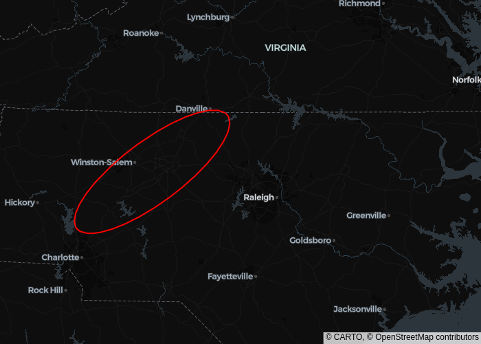
fig = go.Figure(go.Scattermap(mode="markers"))
fig.update_layout(
    margin={'r':0,'t':0,'l':0,'b':0},
    map = {
        'style': "dark",
        'center': {'lon': -79, 'lat': 36 },
        'zoom': 6.5
    },
)

x_center = -80  # Example longitude
y_center = 36    # Example latitude
a = 1            # Semi-major axis (in degrees of lat/lon, approximate)
b = 0.3            # Semi-minor axis (in degrees of lat/lon, approximate)
angle = 30      # Rotation angle

x, y = ellipse(x_center, y_center, angle, a, b)

fig.add_trace(go.Scattermap(
    mode="lines",
    lon=x,
    lat=y,
    marker={'size': 10},
    line={'color': 'red'}
))

fig.show()

png

Emitter Geolocation

References