Array Processing - Beamforming & Direction Finding

Est. read time: 6 minutes | Last updated: April 13, 2025 by John Gentile

Contents

Deterministic Beamforming
- Uniform Linear Array (ULA)
- Array Effects
Broadband Beamforming
Adaptive Beamforming
Direction of Arrival (DOA) Estimation
- Monopulse Systems
- DoA References
Distributed Beamforming/DoA
References

import numpy as np
import matplotlib.pyplot as plt
from matplotlib import cm
import scipy.constants

from IPython.display import YouTubeVideo

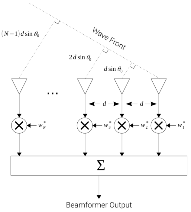
Filtering is a commonly used operation in signal processing; in the discrete sense, samples are passed through a set of filter coefficients, or “taps”, to perform the convolution and achieve the desired response. Analogous to such temporal filtering, an array of sensors can be filtered spatially to produce a desired response across the elements.

Specifically in the context of Radio Frequency (RF) antenna arrays, this spatial filtering can be utilized to optimize the overall antenna pattern, in a process commonly known as beamforming. The specific spatial optimization is often application dependent, however beamforming is generally seen as a method of beam steering, where gain is provided in a specific, desired direction- relative to the array’s front-, with attenuation in other angles. Though the term “beamforming” sounds specific to transmitting applications- like radiating RF arrays-, beamforming, and consequently spatial filtering, can actually be performed on both the transmit and receive functions of any array, also known as array reciprocity. Beamforming is inclusive of non-RF arrays and applications as well, such as sound transducers used in SONAR arrays.

The fundamental operation of beamforming is derived from the properties of constructive and destructive interference of propagating waves in phased array systems. These systems are so named in that the individual array elements shift the phase of a received, or transmitted, signal to create a desired far field array pattern that culminates into a steered wavefront.

This phase shifting process can be achieved by digital or analog means; analog phase shifter units can perform the beam steering in the RF/analog domain. In this case, each phase shifter unit is attached to an individual array antenna element, and is manifolded to a single receiver- such as an Analog to Digital Converter (ADC)- and/or a single transmitter- such as a Digital to Analog Converter (DAC). The benefits of such a system is simplicity in the digital and RF electronics, as there is only one ADC and/or DAC- and possibly one mixing/heterodyne system for the array-, however the system is much less flexible in that it can only steer in one direction at a time.

However for Multiple-Input Multiple-Output (MIMO) or other systems that need more flexibility, these phase shifting blocks could also be performed in the digital domain. In this case, each antenna element can be considered to be directly connected to an ADC and/or DAC and the associated phase shifts can be performed in digital logic- such as in a Field-Programmable Gate Array (FPGA) directly connected to each ADC/DAC- and then coherently combined to form the intended beam(s). The downside of a digitally beamformed system is increased complexity- and thereby often an increased cost- due to each channel requiring RF and sampling electronics that must be phase synchronous, however the upside is this system is much more flexible in how it can apply phase shifts, as well as it creates the opportunity for a system to create multiple spatial beams at one time.

For MIMO communication arrays, these properties of directional gain and attenuation can be exploited for servicing multiple users, such as in Spatial Multiplexing, where distinct users are assumed to be in different spatial locations or directions, so digital beamforming with multiple beams can be used to target each user independently at the same time.

Deterministic Beamforming

Uniform Linear Array (ULA)

A ULA is defined as an array with $N$ elements equally spaced a distance $d$ from each other along a linear axis. Each RF channel- related to an RF antenna element- is sampled synchronously such that the digital samples are aligned in time across all channels so coherent processing can be performed. It can be seen that when dealing with a signal from the far field impinging on the array with angle, $\theta_{0}$ , the difference in propagation path length, $L$ , between elements in a ULA is given by:

L(n) = nd\sin(\theta_{0}), \quad 0 \leq n \leq N - 1

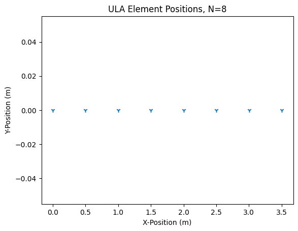
Set the parameters and system constants for the Uniform Linear Array (ULA), including the number of antenna elements, $N$ , the operating/carrier frequency, $f_{c}$ , and the desired plane wave angle of arrival (AoA) relative to boresight, $\theta_{0}$ :

N       = 8     # number of elements in ULA
fc      = 300e6 # RF carrier frequency (assuming narrowband here)
fs      = 1e9   # IF/direct sampling frequency
theta   = -10   # desired signal Angle of Arrival (AoA) in degrees
SNR     = 1     # element SNR (linear units)
noiseP  = 1     # noise power (linear units)
spacing = 0.5   # d/wavelength element spacing (0.5 = half-wavelength spacing)

wavelength = fc/scipy.constants.c
# generate array of antenna element positions
antPos = np.linspace(0,N-1,N)*wavelength*spacing
plt.scatter(antPos, np.zeros(N), marker='1')
plt.title("ULA Element Positions, N=%i" % N)
plt.ylabel("Y-Position (m)")
plt.xlabel("X-Position (m)")
plt.show()

png

For narrowband signals, the complex spatial response vector is formed from the baseband envelope phasor at each ULA element, which is a function of AoA $\theta_{0}$ , operating wavelength $\lambda$ , and the elemental spacing $d$ :

s_{n} = e^{j 2\pi (n-1) \frac{d}{\lambda} \sin{\theta_{0}} } \quad 0 \leq n \leq N - 1

# given wavelength (same units as ula_pos_vec), azimuth direction of wave impinging on ULA, and N-element antenna position vector
def narrowband_spatial_phasor(wavelen, theta_deg, ula_pos_vec):
    cmplx_pos = (1j*2*np.pi/wavelen)*ula_pos_vec.T
    sn = np.exp(cmplx_pos*np.sin(np.deg2rad(theta_deg)))
    return sn
    
s = narrowband_spatial_phasor(wavelength, theta, antPos)

Compute hypothesis of steering vectors in sine space for quiescent beamforming weights. Plot the weight response over sine space by testing weight magnitude at each look direction in vector u, from $-90^{\circ}$ to $90^{\circ}$

# numHyp = number of direction hypothesis to compute
def calc_quiescent_weights(wavelen, ula_pos_vec, numHyp=400):
    u = np.linspace(-1, 1, numHyp)
    wq = np.exp(np.outer((1j*2*np.pi/wavelen)*ula_pos_vec.T, u))
    # normalize quiescent filter weights to unity (0dB) @ boresight
    mag = wq * wq.conj()
    wq = wq / mag.sum(axis=0) # sum over columns (each channel, per hypothesis)
    return wq, u

wq, u = calc_quiescent_weights(wavelength, antPos, 400)

def plot_az_cut(weights,                 # weights to plot
                thetas,                  # list of tuples (angles, wavelengths)
                                         # to plot (1st is desired angle)
                plt_title='Azimuth Cut', # plot title
                lims=[-40,1]):           # plot limits (b/c resp -> 0 near edges)
    # convolve quiescent ULA response w/given spatial weights
    conv_weights = np.inner(wq.conj().T, weights)
    fig, ax = plt.subplots()
    ax.plot(u*spacing, 20*np.log10(np.abs(conv_weights)), linewidth=0.5)
    ax.set(xlabel=r'Normalized Angle, $\frac{d}{\lambda} \sin(\theta)$',
           ylabel='Magnitude (dB)',
           title=plt_title)
    ax.set_ylim(lims)
    for idx, angle in enumerate(thetas):
        if idx == 0:
            lin_color = 'green'
            plt_lbl = r'$\theta_{c}$'
        elif idx == 1:
            lin_color = 'red'
            plt_lbl = r'$\theta_{Inf}$'
        else:
            lin_color = 'red'
            plt_lbl = ''
        # NOTE: since interference tone is at different frequency than desired
        #       tone, the normalized sine space plot scales the incidence angles
        #       by its wavelength
        norm_angle = np.sin(np.deg2rad(angle[0]))*spacing/angle[1]
        # wrap normalized angle for wavelengths >>/<< desired
        while norm_angle < -spacing:
            norm_angle += 2*spacing
        while norm_angle > spacing:
            norm_angle -= 2*spacing
        ax.vlines(norm_angle,
                  lims[0], lims[1],
                  colors=lin_color,
                  linestyles='dashed',
                  label=plt_lbl,
                  linewidth=(3 if idx == 0 else 1))
    ax.legend()
    plt.show()

# create matched filter (beam weights) for quiescent case (no interference)
plot_az_cut(s,
            [(theta, wavelength)],
            plt_title='Azimuth Cut: Quiescent Weight Response in Sine Space',
            lims=[-40, 1])

png

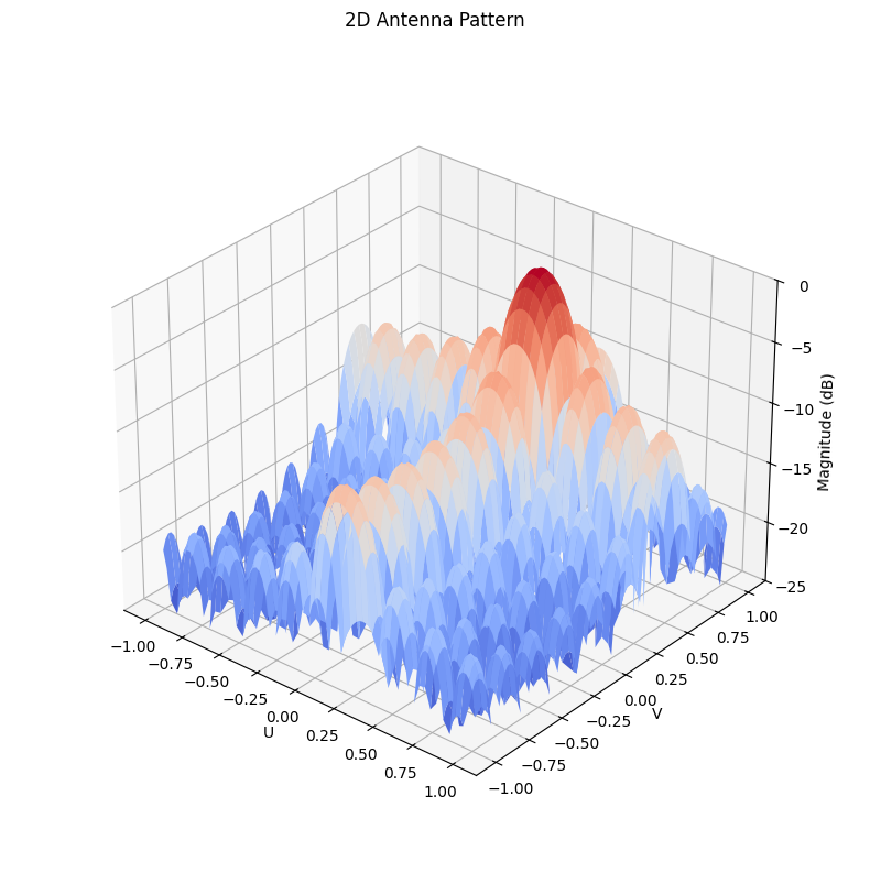
The equation in 2 dimensions, $u$ and $v$ , becomes

\Large F(\theta, \phi) = \sum_{m}^{M} \sum_{n}^{N} \lvert a_{m,n} \rvert \exp{\left\{ j k_0 \left[ m d_x (u - u_0) + n d_y (v - v_0) \right] \right\}}

or if $a_{m,n}$ is separable to $a_{m,n} = b_m c_n$ , then

\Large F(\theta, \phi) = \left\{ \sum b_m \exp{\left[ j k_0 m d_x \left( u - u_0 \right) \right]} \right\} \left\{ \sum c_n \exp{\left[ j k_0 n d_y \left( v - v_0 \right) \right]} \right\}

N = 9  # number of elements in horizontal dimension
M = 9  # number of elements in vertical dimension

n = np.arange(N)  # array for summing over n
m = np.arange(M)  # array for summing over m

d_x = wavelength / 2  # x spacing
d_y = wavelength / 2  # y spacing
k_0 = 2 * np.pi / wavelength # wave number

steering_angle_theta = 10  # theta steering angle
steering_angle_phi = 30  # phi steering angle

u_0 = np.sin(steering_angle_theta * np.pi / 180)  # theta steering angle in sine space
v_0 = np.sin(steering_angle_phi * np.pi / 180)  # phi steering angle in sine space

npts = 100
theta = np.linspace(-np.pi, np.pi, npts)
phi = np.linspace(-np.pi, np.pi, npts)

u2 = np.sin(theta) * np.cos(phi)
v2 = np.sin(theta) * np.sin(phi)

u2 = np.linspace(-1, 1, npts)
v2 = np.linspace(-1, 1, npts)

U, V = np.meshgrid(u2, v2)  # mesh grid of sine space

def compute_af_2d(weights_n, weights_m, d_x, d_y, k_0, u_0, v_0):
    AF_m = np.sum(
        weights_n[:, None, None]
        * np.exp(1j * n[:, None, None] * d_x * k_0 * (U - u_0)),
        axis=0,
    )
    AF_n = np.sum(
        weights_m[:, None, None]
        * np.exp(1j * m[:, None, None] * d_y * k_0 * (V - v_0)),
        axis=0,
    )

    AF = AF_m * AF_n / (M * N)
    return AF

z_min = -25
z_max = 0

weights_n = np.ones(N)
weights_m = np.ones(M)
AF_rect = compute_af_2d(weights_n, weights_m, d_x,d_y,k_0,u_0,v_0)
AF_rect_log = 10 * np.log10(np.abs(AF_rect))
AF_rect_log_mask = np.where(AF_rect_log > z_min, AF_rect_log, np.nan)

fig = plt.figure(figsize=(10, 10))
ax = fig.add_subplot(111, projection="3d")
ax.plot_surface(U, V, AF_rect_log_mask, cmap=cm.coolwarm)
ax.set_zlim(z_min, z_max)
ax.set_title("2D Antenna Pattern")
ax.set_xlabel("U")
ax.set_ylabel("V")
ax.set_zlabel("Magnitude (dB)")
ax.view_init(elev=30, azim=-50, roll=0)
ax.set_box_aspect(None, zoom=0.85)
plt.show()

png

Array Effects

Far-Field

The reason we assume far field characteristics for the majority of work with array systems is to simplify the math and operations; for the case of a phased array receiver in the near field, an RF emitter is so close to the array that the incident angle of the received energy is different for every element due to the spherical wavefront of the source:

However, in the far field, where the same emitter is farther away from the receiving array, the wavefronts become approximately planar, and each receive element sees an equivalent incidence angle, $\theta$ , of the arriving wave:

The specific point at which a given system is operating in the far field is dependent on many factors of the array’s antenna properties, however a general equation can be found based on an array’s antenna diameter, $D$ , and the wavelength of the operating carrier frequency, $\lambda$ :

Far Field > \frac{2D^{2}}{\lambda}

Grating Lobes

The spatial equivalent to the Nyquist frequency in the temporal domain, to prevent spatial aliasing (grating lobes) the antenna element spacing should be $\frac{d}{\lambda} \leq 0.5$ .