Digital Up & Down Conversion

Est. read time: 2 minutes | Last updated: December 17, 2024 by John Gentile

Contents

Spectral Inversion
$f_{s}/4$ Simplification
Transmit Simplification
References

import numpy as np
import matplotlib.pyplot as plt

from rfproto import measurements, nco, plot, sig_gen

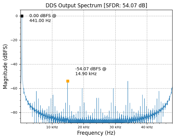
f  = 440.5 # desired output frequency
n  = 48000 # number of output points to compute
fs = 48000 # sampling frequency
N  = 32    # phase accumulator length (num bits)
P  = 9     # LUT table address length (total depth = 2^P)
M  = 16    # quantized word length (num bits)

test_NCO = nco.Nco(N, M, P, fs)

y = np.zeros(n) + 1j*np.zeros(n)
test_NCO.SetOutputFreq(f)
for i in range (n):
    # just take imag part (starts at 0) for this
    y[i] = test_NCO.Step()

plot.spec_an(y, fs, "DDS Output Spectrum", scale_noise=True, norm=True)
plt.show()

png

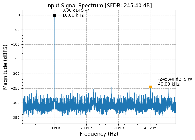
input_sig = sig_gen.cmplx_dt_sinusoid(2**15, 10000, fs, n)
plot.spec_an(input_sig, fs, "Input Signal Spectrum", scale_noise=False, norm=True)
plt.show()

png

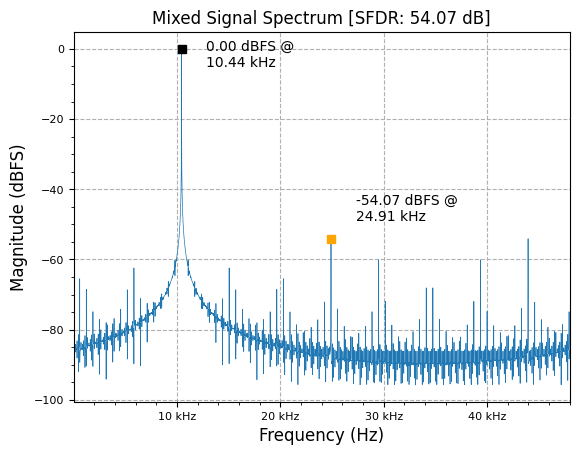
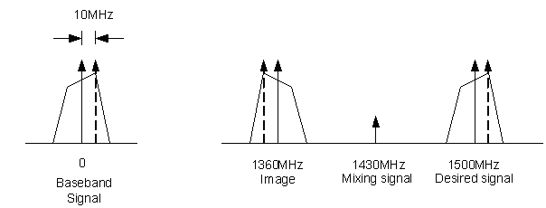
Complex NCO- which acts as discrete-time form of analog heterodyne system’s Local Oscillator (LO)- allows us to mix an input signal up or down in frequency, without worrying about images that would occur with a real-valued NCO (e.g. real valued NCO has frequencies at both $\pm f$ ). The process can be seen as:

A_{NCO}e^{j\omega_{NCO}t} * A_{sig}e^{j\omega{sig}t} = A_{NCO}A_{sig}e^{jt(\omega{sig}+\omega_{NCO})}

It can be seen that mixing adds frequencies, causing an associated shift upwards in total signal output frequency of $f_{NCO} + f_{sig}$ .

mixed = np.zeros(n) + 1j*np.zeros(n)

for i in range(n):
    # NOTE: conj(NCO output) moves mixed signal down, while input * y moves signal up
    mixed[i] = input_sig[i] * y[i]

# NOTE: since both input signal and NCO are complex, there are no images created in mixing
plot.spec_an(mixed, fs, "Mixed Signal Spectrum", scale_noise=False, norm=True)
plt.show()

png

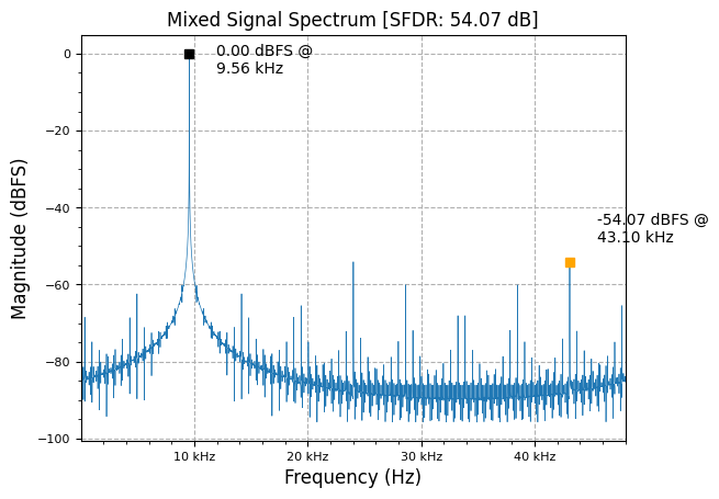
To shift the output frequency down, we can simply take the complex conjugate of the NCO output (e.g. $z=e^{j\omega t}\rightarrow \overline{z}=e^{-j\omega t}$ ) to create a “negative” frequency, since:

\overline{A_{NCO}e^{j\omega_{NCO}t}} * A_{sig}e^{j\omega{sig}t} = A_{NCO}A_{sig}e^{jt(\omega{sig}-\omega_{NCO})}

This mixing subtracts frequencies, causing an associated shift downwards in total signal output frequency of $f_{sig} - f_{NCO}$ .

mixed = np.zeros(n) + 1j*np.zeros(n)

for i in range(n):
    mixed[i] = input_sig[i] * np.conj(y[i])

plot.spec_an(mixed, fs, "Mixed Signal Spectrum", scale_noise=False, norm=True)
plt.show()

png

Spectral Inversion

Based on the mixing process of a signal (both up and down conversion), there exists times where the spectral image is used that inverts the desired spectrum:

To compensate- or generally reverse the direction of rotation- we can simply swap I and Q signals (generally more computationally efficient to multiplying by -1):

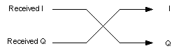
Handling Spectral Inversion in Baseband Processing - Eric Jacobsen

for i in range(len(mixed)):
    mixed[i] = mixed[i].imag + 1j*mixed[i].real

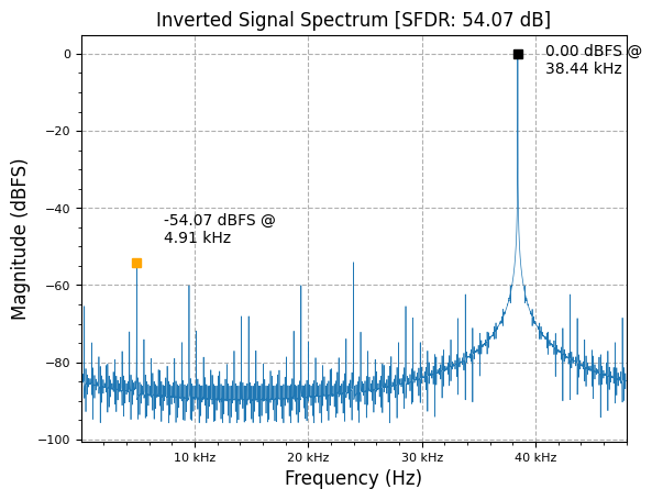
plot.spec_an(mixed, fs, "Inverted Signal Spectrum", scale_noise=False, norm=True)
plt.show()

png

$f_{s}/4$ Simplification

#TODO: when mixer equals $f_{s}/2$ or $f_{s}/4$ , can just use alternating +/-1 (for $f_{s}/2$ ) or +1,0,-1,0 (for $f_{s}/4$ ) very cheaply! Can also be used in lieu of fftshift() type applications.

DSP Trick: Complex Downconverters for Signals at Fs/4 or 3Fs/4 - DSP Guru

Transmit Simplification

Since Digital-to-Analog Converters (DACs) operate on real digital data (real input to real analog output)- except in direct conversion (zero IF) front ends- we only need the real output of a digital upconverter (DUC), either $I$ or $Q$ . In this case, we can simplify the digital mixer (the complex multiplier used to combine the NCO output and transmit I/Q stream) to not have to compute the full complex product (requiring 4x multiplies), but rather just the $I$ term (2x multiplies) as:

Y_{DUC} = (I_{NCO} + jQ_{NCO})(I_{TX} + jQ_{TX})

Y_{DUC} = \underline{(I_{NCO}I_{TX} - Q_{NCO}Q_{TX})} + \cancel{j(I_{NCO}Q_{TX} + I_{TX}Q_{NCO})}

Digital Up & Down Conversion

Spectral Inversion

fs/4f_{s}/4fs​/4 Simplification

Transmit Simplification

References

$f_{s}/4$ Simplification