Filtering Fundamentals

Est. read time: 2 minutes | Last updated: March 02, 2026 by John Gentile

Contents

Filter Design
- Estimate Filter Order
FIR Filters
- Efficient FIR Structures
  - Software Double-Buffering
Windowing
Filter Implementation
- Complex-Valued Filters
- References
Parallel/Vectorized Filter/Convolution
References

import numpy as np
from scipy import signal
import matplotlib.pyplot as plt
from rfproto import utils

Filter Design

Estimate Filter Order

One practical estimate comes from fred harris’ rule-of-thumb:

N_{taps} = \frac{\text{Atten}}{22 * B_{T}}

Where:

$\text{Atten}$ is the desired stopband attenuation, in dB.
$B_{T}$ is the normalized transition band, or $B_{T} = \frac{f_{stop}-f_{pass}}{f_{s}}$

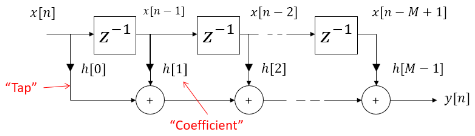
FIR Filters

The discrete-time convolution of $M$ filter coefficients with input samples $x[n]$ can be seen as:

y[n] = x[n] * h[n] = \sum_{k=0}^{M-1}h[k]x[n-k]

Picture link

class fir_filter:
    """Naive class to demonstrate direct-form FIR filtering. If wanting to efficiently compute the direct-form convolution, see [SciPy Signal's lfilter](https://docs.scipy.org/doc/scipy/reference/generated/scipy.signal.lfilter.html)"""

    def __init__(self, h: np.ndarray):
        self.N = len(h)
        self.h = h
        self.dly = np.zeros(self.N)

    def step(self, x: float) -> float:
        # First shift in sample into delay line
        for i in reversed(range(self.N)):
            if i < self.N - 1:
                self.dly[i + 1] = self.dly[i]
        self.dly[0] = x

        # Next multiply and accumulate the discrete convolution of delay line
        # samples and filter tap coefficients
        mac = 0.0
        for i in range(self.N):
            mac += self.dly[i] * self.h[i]
        return mac

    def reset(self):
        self.dly = np.zeros(self.N)

test_filt = fir_filter([0, 0, 1, 0, 0])
for i in range(10):
    print(test_filt.step(i+1))

0.0 0.0 1.0 2.0 3.0 4.0 5.0 6.0 7.0 8.0

Efficient FIR Structures

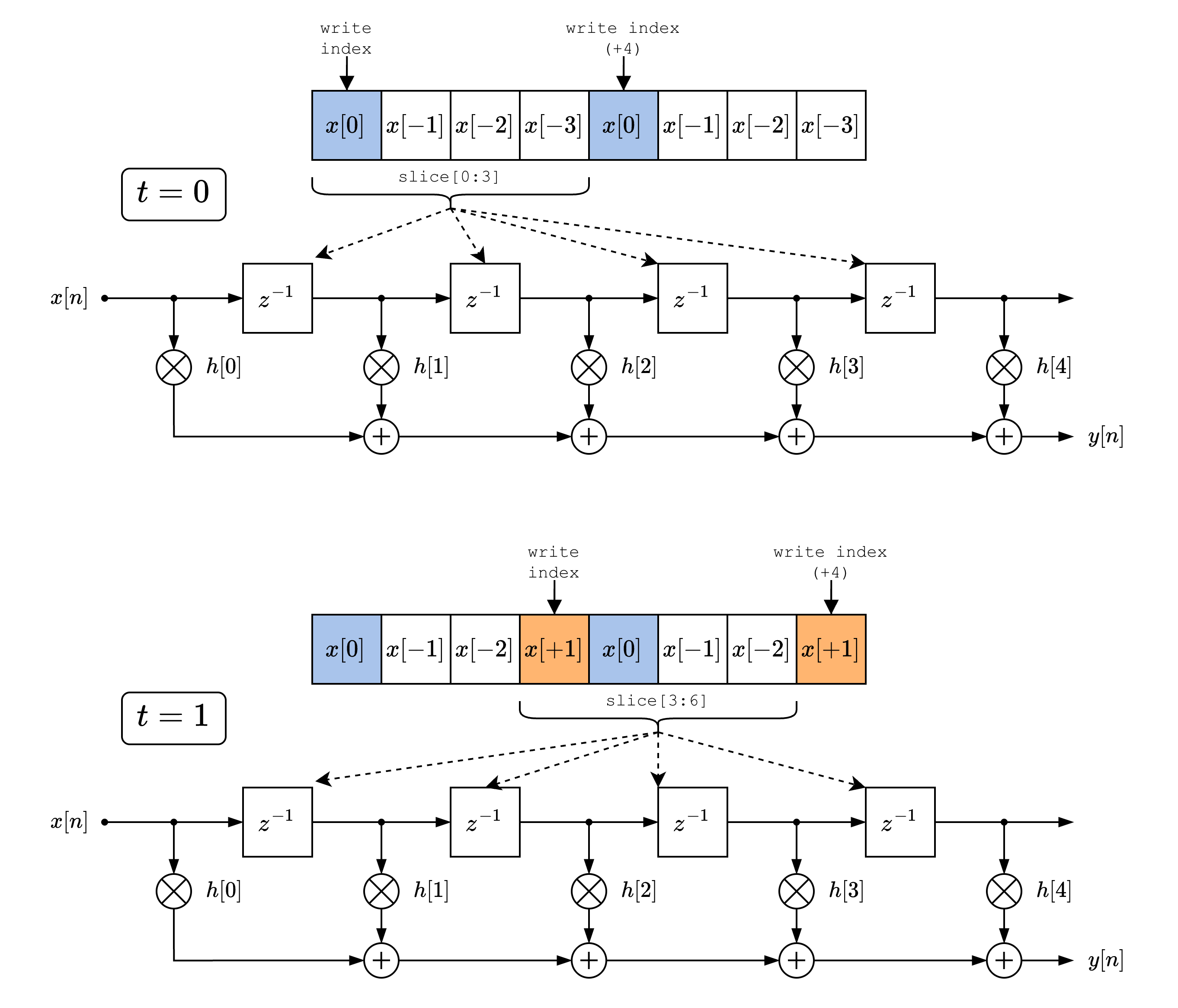
Software Double-Buffering

Shifting sample values within a buffer (e.x. common delay line approach where last value is shifted out, while newest value is shifted in) is very expensive in data movement and cycles. Instead, we can simply double buffer the sample delay line, and write a new sample in two locations- in this way, we can simply shift the a pointer within the double buffer to take a slice during convolution, drastically reducing overhead:

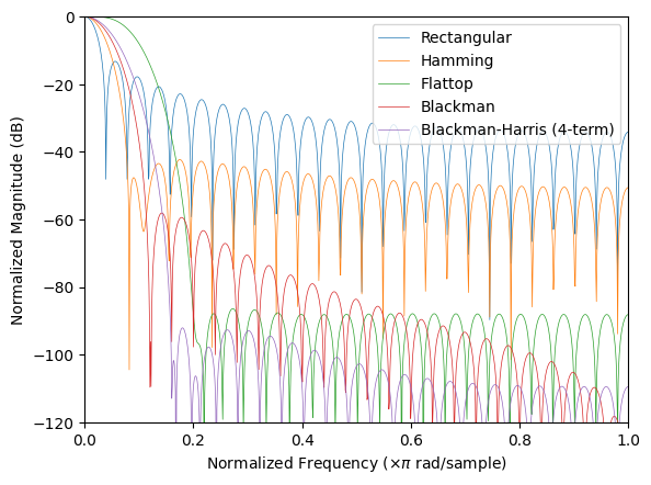
Windowing

Window function - Wikipedia: includes list of window functions with example of time and frequency domain responses.

plt.figure()
num_pts = 51
windows = {}
windows['Rectangular'] = signal.windows.boxcar(num_pts)
windows['Hamming'] = signal.windows.hamming(num_pts)
windows['Flattop'] = signal.windows.flattop(num_pts)
windows['Blackman'] = signal.windows.blackman(num_pts)
windows['Blackman-Harris (4-term)'] = signal.windows.blackmanharris(num_pts)

for window in windows:
    A = np.fft.rfft(windows[window], n=2048) / (num_pts/2.0)
    response = np.abs(A / abs(A).max())
    response = 20 * np.log10(np.maximum(response, 1e-10))
    freq = np.linspace(0, 1, len(response))
    plt.plot(freq, response, label=window, linewidth=0.5)
plt.axis([0, 1.0, -120, 0])
plt.ylabel("Normalized Magnitude (dB)")
plt.xlabel(r"Normalized Frequency ($\times\pi$ rad/sample)")
plt.legend()
plt.show()

png

Filter Implementation

Complex-Valued Filters

Rarely you’ll need to use a complex-valued filter- often you’re looking to apply a filter on complex-valued input signals. In this case, the same real filter tap values and convolution process can happen in parallel on both real and imaginary parts of the signal.

Complex Filter Design

References

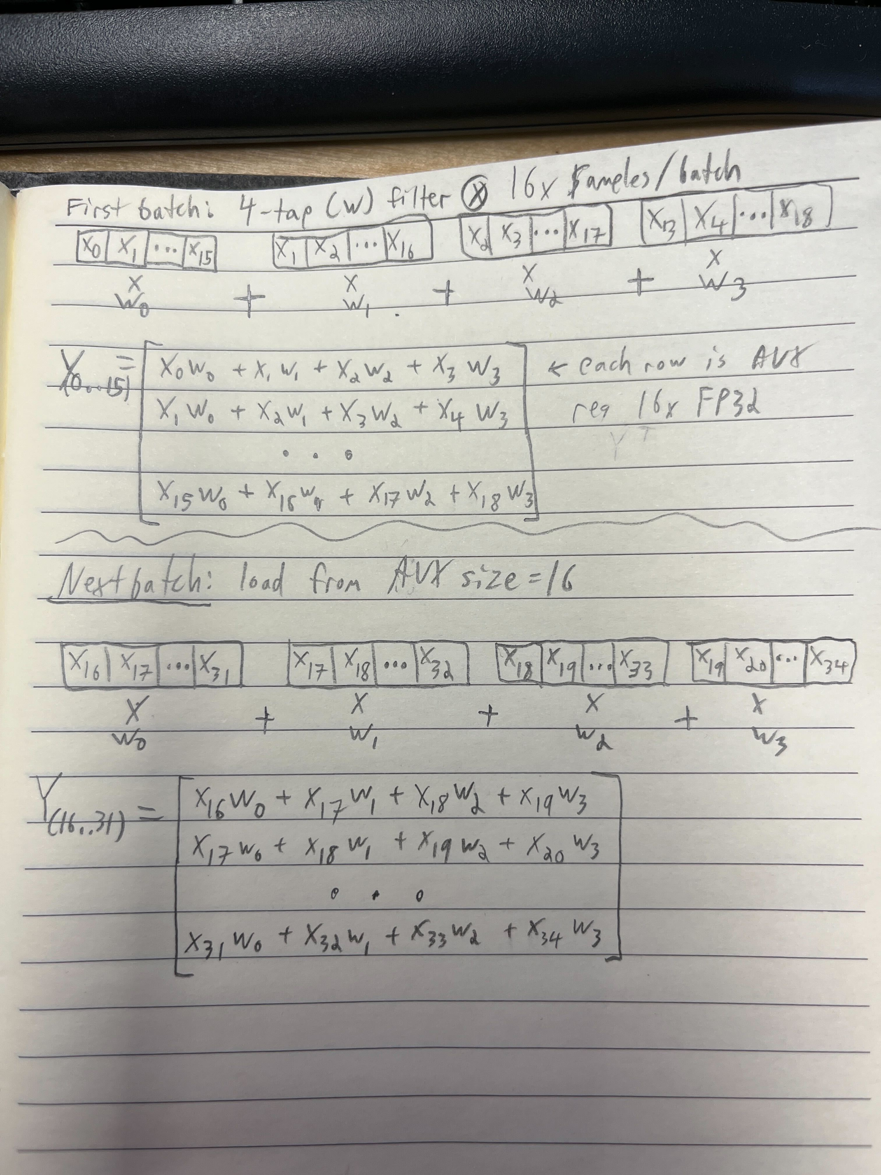
SciPy Signal - Filter Design Methods

Parallel/Vectorized Filter/Convolution

References

DSP: Designing for Optimal Results High-Performance DSP Using Virtex-4 FPGAs: how to design FIR filters in FPGAs for speed and resources based on DSP primitives.
FIR Compiler LogiCORE IP Product Guide (PG149) - AMD Xilinx: notes on Xilinx specific FIR filter IP core, with notes on how different filter structures can be exploited for symmetry, sampling rates, etc.