Timing Synchronization & Timing Error Detectors (TED)

Est. read time: 3 minutes | Last updated: July 17, 2026 by John Gentile

Contents

Timing Error Detector (TED)
- Gardner TED
- Mueller & Muller (M&M) TED
Polyphase Matched Filter for Timing Synchronization
- Harris Polyphase Derivative Matched Filter TED
References

import numpy as np
import matplotlib.pyplot as plt
from scipy import signal
from rfproto import filter, modulation, pi_filter, plot, sig_gen

Timing Error Detector (TED)

# simulate random binary input values
num_symbols  = 2400
sym_rate     = 1e6 # Baseband symbol rate
# Generate random QPSK symbols
rand_symbols = np.random.randint(0, 4, num_symbols)

L  = 2               # Upsample ratio (sim 2x Samples per Symbol)
fs = L * sym_rate    # Output sample rate (Hz)

rolloff          = 0.5 # Alpha of RRC
num_filt_symbols = 6    # Symbol length of RRC matched filter

qpsk_tx_filtered_2x = sig_gen.gen_mod_signal(
    "QPSK",
    rand_symbols,
    fs,
    sym_rate,
    "RRC",
    rolloff,
    num_filt_symbols,
)

# Add timing offset (0.3 samples delay) via fractional delay filter
timing_offset = 0.3
frac_N = 21 # number of taps in fractional filter (should be odd)
frac_idx = np.arange(-(frac_N-1)//2, frac_N//2+1)
frac_h = np.sinc(frac_idx - timing_offset) # calc filter taps
frac_h *= np.hamming(frac_N) # window filter to make sure it decays to 0 on both sides
frac_h /= np.sum(frac_h) # normalize to get unity gain filter weights
samples_rx = np.convolve(qpsk_tx_filtered_2x, frac_h)

# Add AWGN noise
#samples_rx += 0.05 * (np.random.randn(len(samples_rx)) + 1j * np.random.randn(len(samples_rx)))

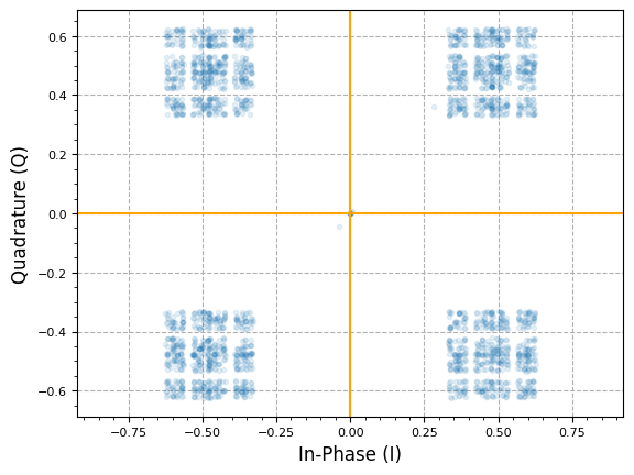
plot.IQ(samples_rx, alpha=0.1)
plt.show()

png

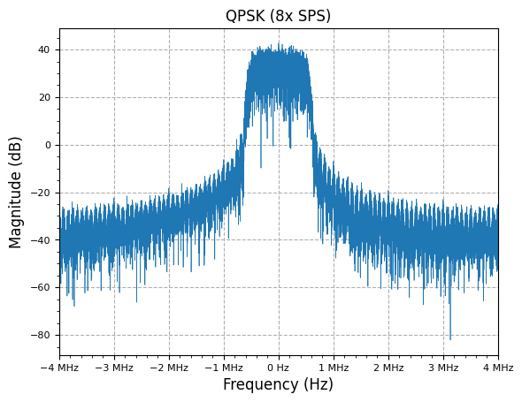
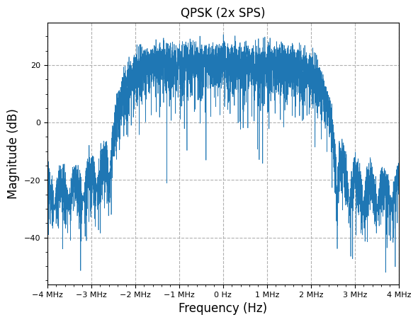
plot.spec_an(samples_rx, fs=fs, fft_shift=True, show_SFDR=False, y_unit="dB", title=f"QPSK ({L}x SPS)")
plt.show()

png

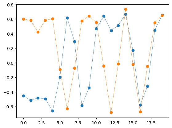
plt.plot(samples_rx[20:40].real, '-o', linewidth=0.5)
plt.plot(qpsk_tx_filtered_2x[20:40].real, '-o', linewidth=0.5)
plt.show()

png

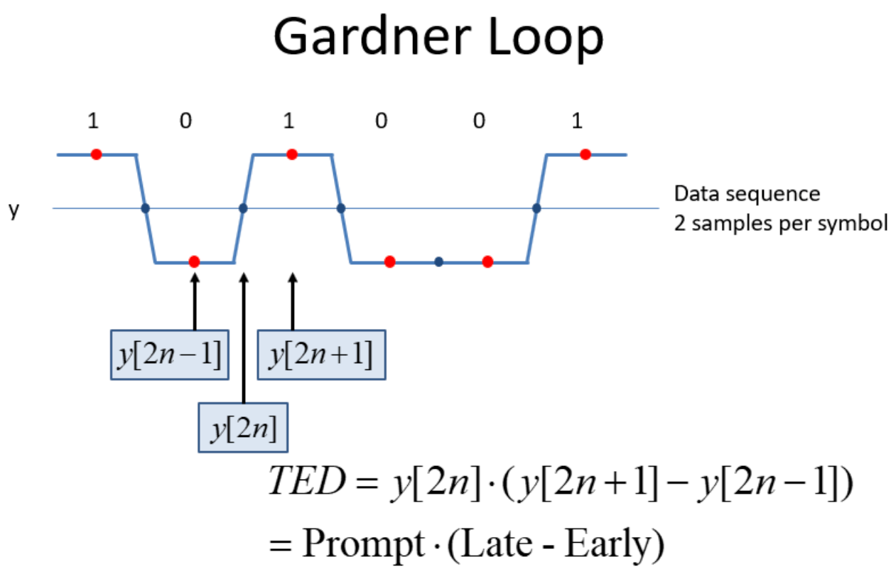
Gardner TED

From this DSP StackExchange Post

e(n) = \mathbb{R}[\overline{y_{n}}(y_{n+1} - y_{n-1})]

early = prompt = late = 0.0 * 1j*0.0
gardner_ted_out = []

# Perform TED error calculation -> real{conj(y[n]) * (y[n+1] - y[n-1])}
#  early (y[2n - 1]), prompt (y[2n]), late (y[2n + 1])
def gardner_ted(early, prompt, late):
    return (np.real(prompt)*(np.real(late)-np.real(early))) + (np.imag(prompt)*(np.imag(late)-np.imag(early)))

for sample in samples_rx[:50]:
    # Shift in samples at 2x SPS rate to TED early/prompt/late registers
    early = prompt # y[2n - 1]
    prompt = late  # y[2n]
    late = sample  # y[2n + 1]
    
    gardner_ted_out.append(gardner_ted(early, prompt, late))

plt.plot(gardner_ted_out, linewidth=0.5)
plt.show()

png

Mueller & Muller (M&M) TED

e(n) = \mathbb{R}[(y_{n} - y_{n-1}) * \overline{\text{sign}(y_{n-1})}] - \mathbb{R}[(\text{sign}(y_{n}) - \text{sign}(y_{n-1})) * \overline{y_{n-1}}]

rrc_coef = filter.RootRaisedCosine(L, 1, rolloff, 2 * num_filt_symbols * L + 1)
samples_rx_post_mf = signal.lfilter(rrc_coef, 1, samples_rx)
# downsample to 1x SPS
samples_rx_post_mf = samples_rx_post_mf[::2]

plot.IQ(samples_rx_post_mf, alpha=0.1)
plt.show()

png

# current (y[n]) and previous (y[n-1])
def mm_ted(curr, prev):
    mm_real = (np.real(curr) * np.sign(np.real(prev))) - (np.real(prev) * np.sign(np.real(curr)))
    mm_imag = (np.imag(curr) * np.sign(np.imag(prev))) - (np.imag(prev) * np.sign(np.imag(curr)))
    return mm_real + mm_imag

mm_out = []
for i in range(1, len(samples_rx_post_mf)):
    mm_out.append(mm_ted(samples_rx_post_mf[i], samples_rx_post_mf[i-1]))

plt.plot(mm_out, linewidth=0.5)
plt.show()

print(f"Mean timing error: {np.mean(mm_out):.4f}")
print(f"Error std dev: {np.std(mm_out):.4f}")

png

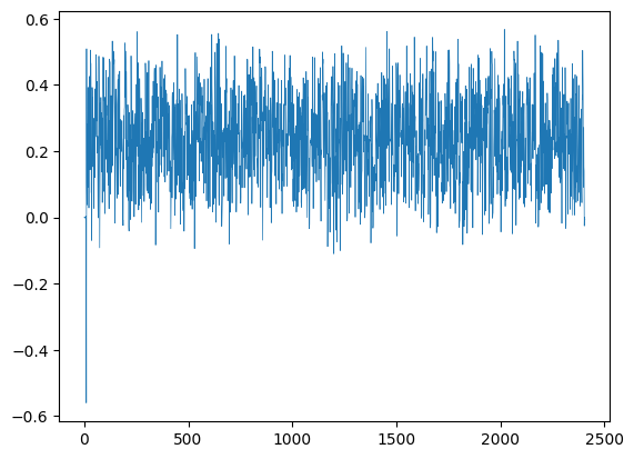
Mean timing error: 0.2331 Error std dev: 0.1265

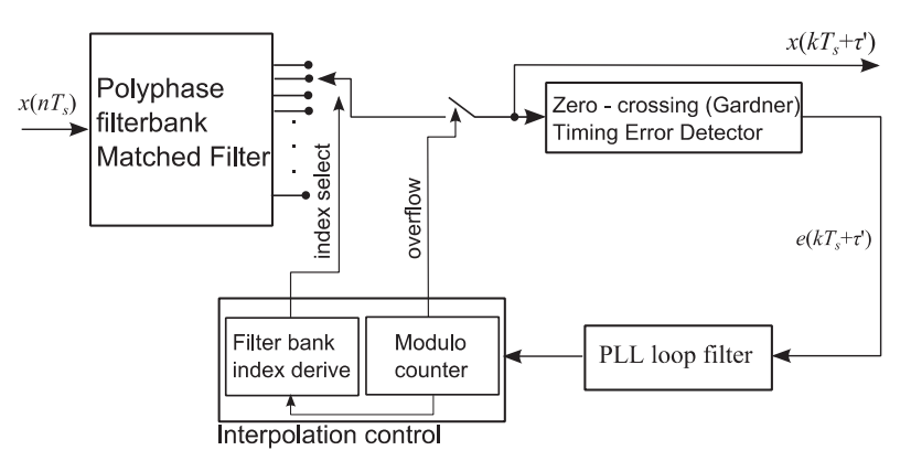
Polyphase Matched Filter for Timing Synchronization

From the Multirate DSP page on Polyphase Filters, we know that each leg of a polyphase filter is an all-pass filter, with each leg providing a fractional amount of signal delay ( $1/M$ samples of delay, where $M$ is the number of polyphase branches), spread equally over the duration of a symbol period. We can exploit this feature by coopting the commutator- traditionally used to cycle through each polyphase leg to perform the interpolation or decimation operation- to act as the delay selector in a timing error correction block!

This also leads to implementation optimizations, as only one FIR filter structure need be instantiated, with the commutator indexing a Look-Up Table (LUT) of each polyphase leg’s filter coefficients at a given time.

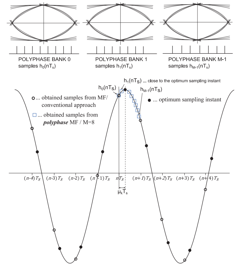
In a simple simulated system above, we were able to generate a QPSK signal (no frequency or phase offset present) at 2x Samples per Symbol (SPS). Below, we will see the ideal sampling location (minimal deviation from ideal constellation points in I/Q plane) can be found after matched filtering with a polyphase filter implementation, selecting a timing offset based off commutator/branch, and final downsampling to 1x SPS.

For the Polyphase Interpolation Filter case, we start by generating a similar Root Raised Cosine (RRC) filter as before, however the prototype filter is scaled by the number of polyphase filter legs- as done in other polyphase prototype designs- to maintain the correct matched filter response.

# The number of taps of this filter is based on how long you expect the channel to be; that is, 
# how many symbols do you want to combine to get the current symbols energy back, usually 5 to 10+
taps = 2 * num_filt_symbols * L + 1
# With 32 filters, you get a good enough resolution in the phase to produce very small, almost 
# unnoticeable, ISI. Going to 64 filters can reduce this more, but after that there is very little 
# gain for the extra complexity. Total prototype filter taps = taps * num_filters, since we're 
# instantiating segments of these taps into the filterbanks in such a way that each bank now 
# represents the filter at different phases, equally spaced at 2pi/N, where N is the number of filters.
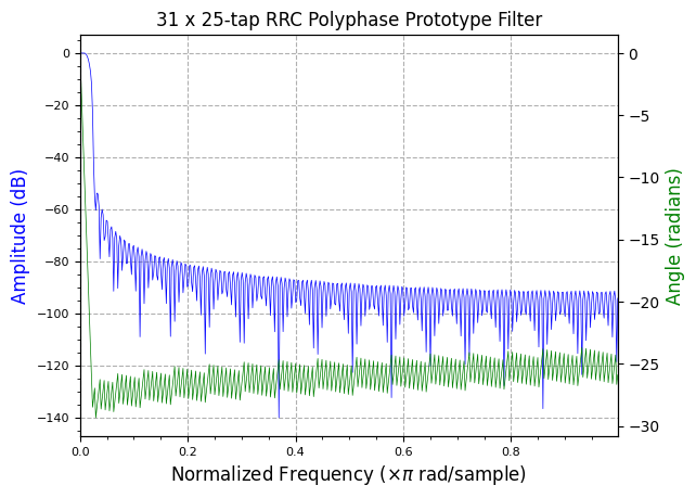
num_filters = 31
polyphase_rrc_coef = filter.RootRaisedCosine(num_filters * L, 1, rolloff, taps * num_filters)

plot.filter_response(polyphase_rrc_coef, title=f"{num_filters} x {taps}-tap RRC Polyphase Prototype Filter")
plot.plt.show()

png

h_poly_rrc = polyphase_rrc_coef.reshape(len(polyphase_rrc_coef)//num_filters, num_filters).T
print(np.shape(h_poly_rrc))

(31, 25)

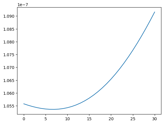
We can then simulate sweeping of the commutator and filtering input samples across each static leg of the RRC polyphase filter to show the eye opening and closing based on timing correction:

from matplotlib.animation import FuncAnimation

fig, ax = plt.subplots()
line, = ax.plot([], [], ".", alpha=0.3)
plt.axvline(x=0, color="orange")
plt.axhline(y=0, color="orange")
plt.margins(x=0)
plt.grid(True, linestyle="--")
plt.minorticks_on()
plt.tick_params(labelsize=8)
plt.xlabel("In-Phase (I)", fontsize=12)
plt.ylabel("Quadrature (Q)", fontsize=12)
ax.set_yticklabels([])
ax.set_xticklabels([])
iq_vhlim = 0.04
ax.set_xlim([-iq_vhlim, iq_vhlim])
ax.set_ylim([-iq_vhlim, iq_vhlim])

def update_plot(frame):
    poly_match_out = signal.lfilter(h_poly_rrc[frame], 1, samples_rx)
    # NOTE: perform final decimation-by-2 here to bring output to 1x SPS
    line.set_xdata(np.real(poly_match_out[::2]))
    line.set_ydata(np.imag(poly_match_out[::2]))
    ax.set_title(f"Polyphase RRC Leg: {frame}")
    return line,

anim = FuncAnimation(fig, update_plot, frames=num_filters, interval=100, blit=True, repeat=True)
anim.save('iq_polyphase_timing.gif', writer='pillow')
plt.close()

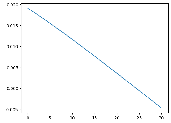
s_curve = []
for i in range(num_filters):
    poly_match_out = signal.lfilter(h_poly_rrc[i], 1, samples_rx)
    temp = 0.0
    for j in range(1, len(poly_match_out) - 1):
        temp += gardner_ted(poly_match_out[j-1], poly_match_out[j], poly_match_out[j+1])
    temp /= len(poly_match_out)
    s_curve.append(temp)
plt.plot(s_curve)
plt.show()

png

s_curve = []
for i in range(num_filters):
    poly_match_out = signal.lfilter(h_poly_rrc[i], 1, samples_rx)
    poly_match_out = poly_match_out[::2]
    temp = 0.0
    for j in range(1, len(poly_match_out)):
        temp += mm_ted(poly_match_out[j], poly_match_out[j-1])
    temp /= len(poly_match_out)
    s_curve.append(temp)
plt.plot(s_curve)
plt.show()

png

in_delay = np.zeros(taps) * 1j*np.zeros(taps)
prev = 0.0 * 1j*0.0
filt_out = []
ted_out = []
pi_out = []
comm_idx = 0
loop_filt = pi_filter.PiFilter(frac_loop_bw=0.001, detector_gain=1e-5)
# set initial loop filter value to mid point of polyphase branches
loop_filt.accumulator = num_filters // 2

for idx, x in enumerate(samples_rx):
    # First shift in sample into delay line
    for i in reversed(range(taps)):
        if i < taps - 1:
            in_delay[i+1] = in_delay[i]
    in_delay[0] = x

    # Next multiply-accumulate the discrete convolution of delay line of input
    # samples with the current polyphase filter leg coefficients
    mac = 0.0 * 1j*0.0
    for i in range(taps):
        mac += in_delay[i] * h_poly_rrc[comm_idx][i]

    filt_out.append(mac)
    
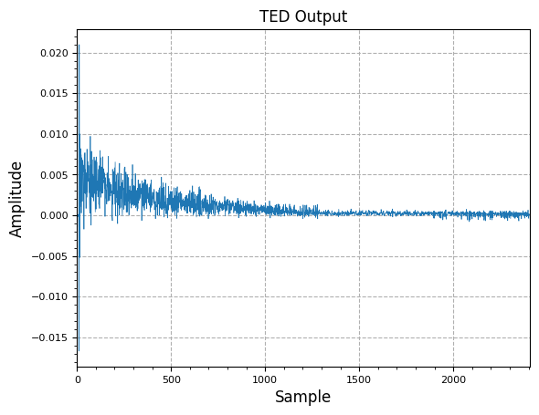
    if idx % 2 == 0:
        err = mm_ted(mac, prev)
        ted_out.append(err)
        prev = mac

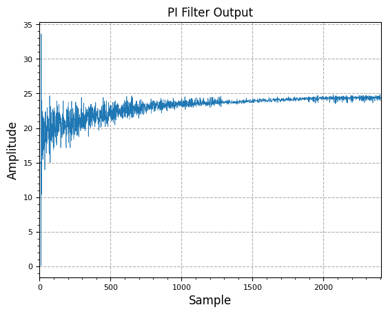
        # Loop filter
        pi_tmp = loop_filt.Step(err)
        pi_out.append(pi_tmp)
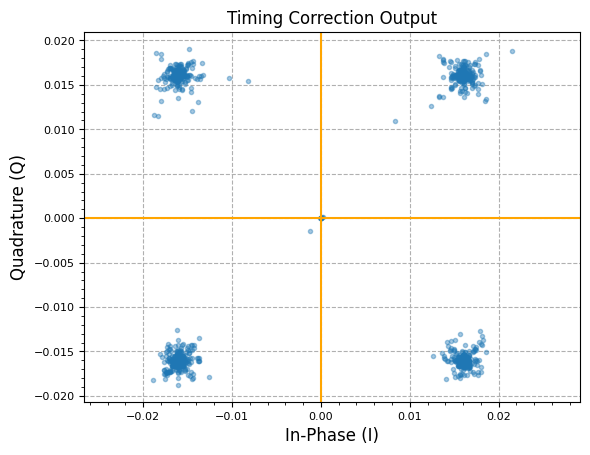
        comm_idx = round(pi_tmp) % num_filters

plot.IQ(filt_out[::2], alpha=0.4, title="Timing Correction Output")
plt.show()

plot.samples(ted_out, title="TED Output")
plt.show()

plot.samples(pi_out, title="PI Filter Output")
plt.show()

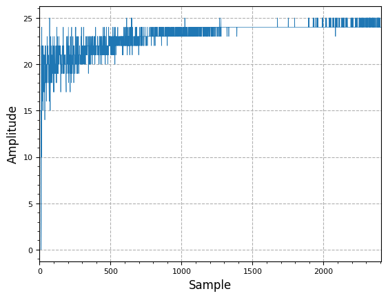
plot.samples(np.round(pi_out) % num_filters)
plt.show()

png

Harris Polyphase Derivative Matched Filter TED

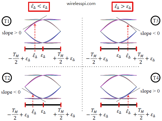
The M&M loop above derives its timing error from the shape of a single matched-filter output stream. The classic fred harris approach is more direct: run a matched filter (MF) polyphase bank alongside a derivative matched filter (DMF) bank, with both banks driven by the same commutator / arm-select index. At the maximum-likelihood (peak) sampling instant the MF output is maximized, so its derivative — the DMF output — passes through zero. The DMF output, sign-corrected by the current symbol decision, is therefore a direct, near-linear estimate of the timing error:

e[n] = \text{sign}\big(\Re\{y_{MF}[n]\}\big)\,\Re\{y_{DMF}[n]\} + \text{sign}\big(\Im\{y_{MF}[n]\}\big)\,\Im\{y_{DMF}[n]\}

We build the DMF bank by taking the central-difference derivative of the same RRC polyphase prototype (np.gradient) and partitioning it into the same $M = 31$ arms — see the Derivative Matched Filter section of the Pulse-Shaping notebook for why the cheap finite-difference derivative is indistinguishable from an ideal $j\omega$ differentiator here (the prototype is heavily oversampled by its polyphase arms, so the signal band sits far below Nyquist). Both banks convolve the same 2x-SPS input delay line each sample; once per symbol the error $e[n]$ drives a PI loop filter whose accumulator is the arm-select index, steering the fractional delay until the constellation is optimally sampled, then decimated from 2x to 1x SPS.

Note this ideal simulation only injects a static fractional (sub-sample) timing offset, so the loop locks by settling on a single polyphase arm; a real link with a clock-frequency offset would additionally slip the integer sample index whenever the arm accumulator wraps past arm $0$ or $M-1$ .

# --- Derivative matched-filter (DMF) polyphase bank ---
# Build the DMF prototype as the central-difference derivative of the SAME RRC
# prototype (np.gradient; see the DMF section of the Pulse-Shaping notebook), then
# partition it into the same number of arms. Arm k of the MF and DMF banks are thus
# selected by one shared commutator/arm-select index.
dproto_rrc = np.gradient(polyphase_rrc_coef)
h_poly_drrc = dproto_rrc.reshape(len(dproto_rrc) // num_filters, num_filters).T

# Decision-directed maximum-likelihood timing error: the symbol decision sign(y_MF)
# picks the QPSK quadrant, and the derivative-MF output y_DMF supplies the slope,
# which is zero at the optimum (peak) sampling instant.
def dmf_ted(y_mf, y_dmf):
    return np.sign(np.real(y_mf)) * np.real(y_dmf) + np.sign(np.imag(y_mf)) * np.imag(y_dmf)

in_delay = np.zeros(taps, dtype=complex)
mf_out, ted_out, pi_out = [], [], []
comm_idx = 0
# detector_gain ~ the S-curve (TED) slope per arm near lock; the PI accumulator
# holds the arm-select index, so we seed it at the middle of the bank.
loop_filt = pi_filter.PiFilter(frac_loop_bw=0.01, detector_gain=3.2e-5)
loop_filt.accumulator = num_filters // 2

for idx, x in enumerate(samples_rx):
    # shift the newest 2x-SPS sample into the shared input delay line
    in_delay[1:] = in_delay[:-1]
    in_delay[0] = x

    # both banks convolve the same delay line, indexed by the same arm select
    y_mf = np.dot(in_delay, h_poly_rrc[comm_idx])    # matched filter
    y_dmf = np.dot(in_delay, h_poly_drrc[comm_idx])  # derivative matched filter
    mf_out.append(y_mf)

    # update the timing loop once per symbol (2x SPS in -> 1x SPS out)
    if idx % 2 == 0:
        err = dmf_ted(y_mf, y_dmf)
        ted_out.append(err)
        pi_tmp = loop_filt.Step(err)
        pi_out.append(pi_tmp)
        comm_idx = int(round(pi_tmp)) % num_filters  # arm select == fractional delay

sym_out = np.array(mf_out[::2])  # decimate to 1x SPS at the symbol instants

# skip the loop acquisition transient so the settled constellation is clear
settle = 400
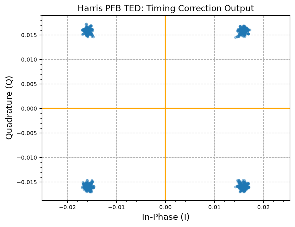
plot.IQ(sym_out[settle:], alpha=0.4, title="Harris PFB TED: Timing Correction Output")
plt.show()

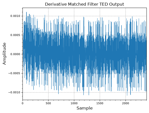
plot.samples(ted_out, title="Derivative Matched Filter TED Output")
plt.show()

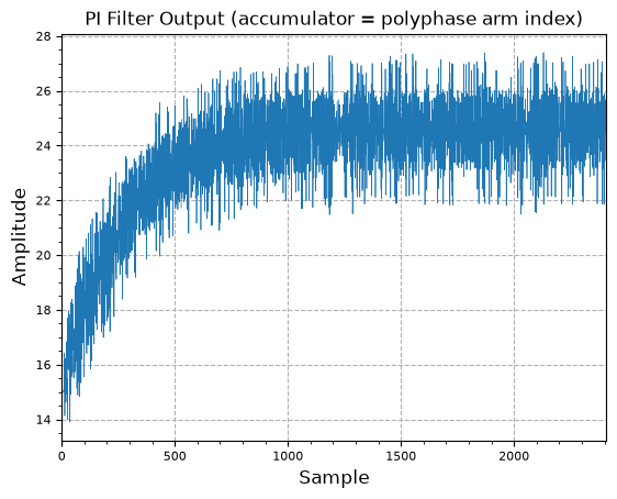
plot.samples(pi_out, title="PI Filter Output (accumulator = polyphase arm index)")
plt.show()

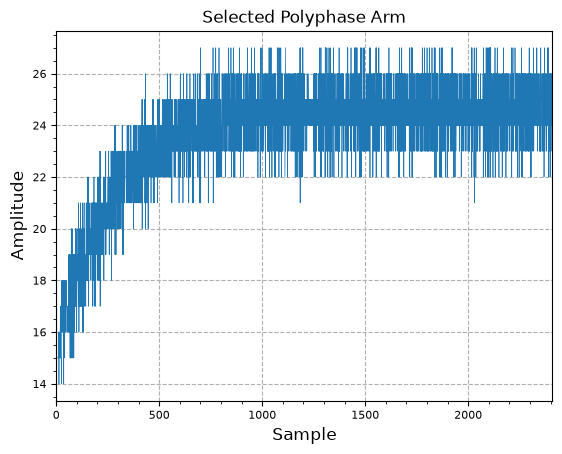
plot.samples(np.round(pi_out) % num_filters, title="Selected Polyphase Arm")
plt.show()

png