End-to-End Machine Learning Example- California Housing Prices

Est. read time: 3 minutes | Last updated: July 17, 2024 by John Gentile

Contents

Model Approach
- Performance Measure
Dataset Creation
- Dataset Download
- Creating Test Set

Here we’ll use housing price dataset from the 1990 CA census from StatLib repository which contains metric such as population, income, and housing price for each block group (the smallest geographical unit for which the census publishes sample data, typically 600 to 3,000 people). Our goal is for our ML model to accurately predict the median housing price in any district, given all other metrics.

Model Approach

Since we are given labeled training examples (accurate census sample data which gives the expected output- median housing price- for each set of features), we can conclude that this is definitely a supervised learning task. Since we are looking to predict a value, it is a regression task, but more specifically, a multiple regression proble, since we need to consider multiple features to make the output prediction (e.g. features like population, median income, etc.). It is also considered a univariate regression problem since we only need to predict a single value for each district; conversely if we needed to predict multiple values, it would be a multivariate regression problem. Finally, since data is not continuously streaming into the system and the dataset is small enough to fit in memory, batch learning is fine for this model.

Performance Measure

Typical for regression problems, we will use the Root Mean Square Error (RMSE) measurement to give an idea of how much error the system is making with predictions at any given time. RMSE is calculated by:

RMSE(\boldsymbol{X},h) = \sqrt{ \frac{1}{m} \sum^{m}_{i=1} \left (h(\boldsymbol{x}^{(i)}) - y^{(i)} \right )^{2} }

Where:

$m$ is the number of samples in the dataset being currently measured
$\boldsymbol{x^{(i)}}$ $x^{(i)}$ is a vector of all feature values (excluding label, $y^{(i)}$ $y^{(i)}$ ) of the i-th instance in the dataset
- For instance, if a district in the dataset has a longitude location of -118.29deg, latitude of 33.91deg, population of 1416, and a median income of $38,372 - with the label/median house value of $156,400- then the vector and label would look like:

\boldsymbol{x^{(i)}} = \begin{pmatrix} -118.29 \\ 33.91 \\ 1416 \\ 38372 \end{pmatrix}

y^{(1)} = 156400

$\boldsymbol{X}$ is the matrix containing all feature values (excluding labels) for all instances in the dataset, which with the above example values, looks like:

\boldsymbol{X} = \begin{bmatrix} \left ( \boldsymbol{x^{(1)}} \right )^{T} \\ \left ( \boldsymbol{x^{(2)}} \right )^{T} \\ \vdots \\ \left ( \boldsymbol{x^{(N)}} \right )^{T} \\ \end{bmatrix} = \begin{pmatrix} -118.29 & 33.91 & 1416 & 38372 \\ \vdots & \vdots & \vdots & \vdots \end{pmatrix}

$h$ is the system’s prediction function (aka hypothesis); it’s the system’s output given a feature vector $\boldsymbol{x}^{(i)}$ , $\hat{y}^{(i)}=h(\boldsymbol{x}^{(i)})$

Once could use another performance function which measures deltas between the prediction vectors and target value vectors, called Mean Absolute Error (MAE):

MAE(\boldsymbol{X},h) = \frac{1}{m}\sum^{m}_{i=1}\left | h(\boldsymbol{x}^{(i)} - y^{(i)} \right |

These various distance measures are also called norms:

Computing RMSE corresponds to the Euclidean norm, or the $\ell_{2}$ norm, denoted colloquially as $\begin{Vmatrix} \cdot \end{Vmatrix}$ (or $\begin{Vmatrix} \cdot \end{Vmatrix}_{2}$ more specifically)
Computing MAE correspongs to the Manhattan norm (because it can measure the distance between two city points where you can only travel in orthogonal blocks), or the $\ell_{1}$ norm, denoted $\begin{Vmatrix} \cdot \end{Vmatrix}_{1}$

In general, the $\ell_{k}$ norm of a vector $\boldsymbol{v}$ containing $n$ elements is defined as:

\begin{Vmatrix} v \end{Vmatrix}_{k} = \left ( |v_{0}|^{k} + |v_{1}|^{k} + \dotsb + |v_{n}|^{k} \right )^{1/k}

The higher the norm index, the more it focuses on large values and neglects small ones, hence why RMSE is more sensitive to outliers than MAE, however when outliers are exponentially rare, RMSE performs very well and is preferred.

Dataset Creation

Dataset Download

Here we will download the comma-separated values (CSV) file that contains our housing dataset, and load it into memory using pandas.

import os
import tarfile
import urllib
import pandas as pd

DL_FOLDER    = "https://raw.githubusercontent.com/ageron/handson-ml2/master/"
HOUSING_PATH = os.path.join("datasets", "housing")
HOUSING_URL  = DL_FOLDER + "datasets/housing/housing.tgz"

# create function to easily download & extract housing dataset tarball
def fetch_housing_data(housing_url=HOUSING_URL, housing_path=HOUSING_PATH):
    os.makedirs(housing_path, exist_ok=True)
    tgz_path = os.path.join(housing_path, "housing.tgz")
    urllib.request.urlretrieve(housing_url, tgz_path)
    housing_tgz = tarfile.open(tgz_path)
    housing_tgz.extractall(path=housing_path)
    housing_tgz.close()
    
def load_housing_data(housing_path=HOUSING_PATH):
    csv_path = os.path.join(housing_path, "housing.csv")
    return pd.read_csv(csv_path)
    
fetch_housing_data() # download now
housing = load_housing_data()
housing.describe() # show a summary of the numerical attributes

	longitude	latitude	housing_median_age	total_rooms	total_bedrooms	population	households	median_income	median_house_value
count	20640.000000	20640.000000	20640.000000	20640.000000	20433.000000	20640.000000	20640.000000	20640.000000	20640.000000
mean	-119.569704	35.631861	28.639486	2635.763081	537.870553	1425.476744	499.539680	3.870671	206855.816909
std	2.003532	2.135952	12.585558	2181.615252	421.385070	1132.462122	382.329753	1.899822	115395.615874
min	-124.350000	32.540000	1.000000	2.000000	1.000000	3.000000	1.000000	0.499900	14999.000000
25%	-121.800000	33.930000	18.000000	1447.750000	296.000000	787.000000	280.000000	2.563400	119600.000000
50%	-118.490000	34.260000	29.000000	2127.000000	435.000000	1166.000000	409.000000	3.534800	179700.000000
75%	-118.010000	37.710000	37.000000	3148.000000	647.000000	1725.000000	605.000000	4.743250	264725.000000
max	-114.310000	41.950000	52.000000	39320.000000	6445.000000	35682.000000	6082.000000	15.000100	500001.000000

# render plots within notebook itself
%matplotlib inline 
import matplotlib.pyplot as plt

housing.hist(bins=50, figsize=(20,15))
plt.show()

png

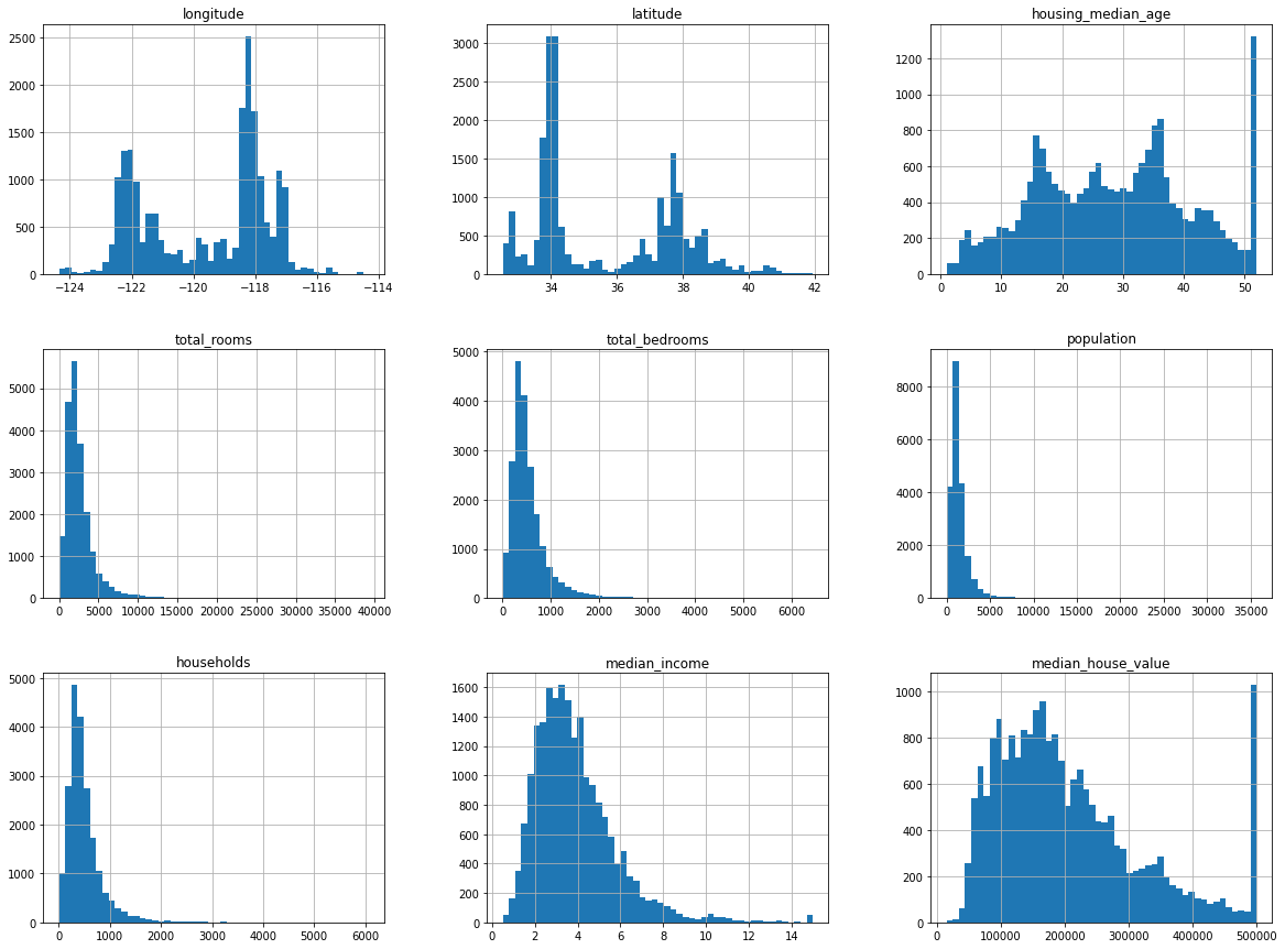
Note that in the above histogram plots, there are a couple important points:

median_income values were normalized to values between 0.5 and 15 (e.g. a value of 3 is equivalent to about $30k). This preprocessing is fine, and common in ML tasks.
housing_median_age and median_house_value values are capped, which may cause an issue since the house value is our target attribute (label), and you don’t want the ML model to learn that prices never go above that limit.
Attributes have very different scales, which we’ll need to tackle with feature scaling.
Many of the plots are tail-heavy (the distribution of values is not symmetrical about the mean) which can be difficult for some ML algorithms to detect patterns.

Creating Test Set

Creating a test set could be as simple as picking some random subset of the dataset (usually around 20%, or less with larger datasets) and set them aside:

import numpy as np

def split_train_test(data, test_ratio):
    shuffled_idx  = np.random.permutation(len(data))
    test_set_size = int(len(data) * test_ratio)
    test_idx      = shuffled_idx[:test_set_size]
    train_idx     = shuffled_idx[test_set_size:]
    return data.iloc[train_idx], data.iloc[test_idx]

train_set, test_set = split_train_test(housing, 0.2)
print("Training dataset size: %d" % len(train_set))
print("Testing dataset size: %d" % len(test_set))

Training dataset size: 16512 Testing dataset size: 4128

While the above works, each time you run the code, a different test data set is generated; over time this means your model will see the whole dataset, which you want to avoid. One way to prevent this would be to set the random number generator’s seed (e.x. np.random.seed()) before calling np.random.permutation().