Basic Radar

Est. read time: 1 minute | Last updated: October 21, 2024 by John Gentile

Contents

References

import random
import numpy as np

from rfproto import plot, impairments, sig_gen

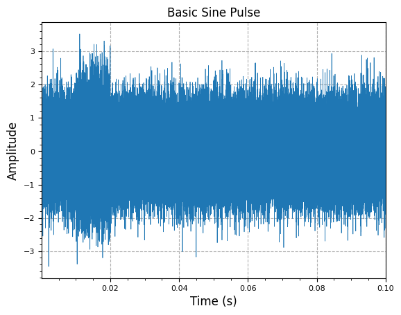
Create a basic pulse of the form:

y(t) = A \cos ( 2\pi f t + \phi)

# time vector based on sampling frequency
fs       = 1e6  # sampling frequency (Hz)
rx_swath = 1e-1 # RX Swath length (seconds)
num_samp = int(np.ceil(fs * rx_swath))  # number of RX samples

# fast time vector
t = np.linspace(1,num_samp,num_samp)/fs
y = impairments.awgn(0.1, len(t))
y[int(0.1*num_samp):int(0.2*num_samp)] += sig_gen.cmplx_ct_sinusoid(1, 3e5, t[:int(0.1*num_samp)])
plot.time_sig(t, y.real, "Basic Sine Pulse")
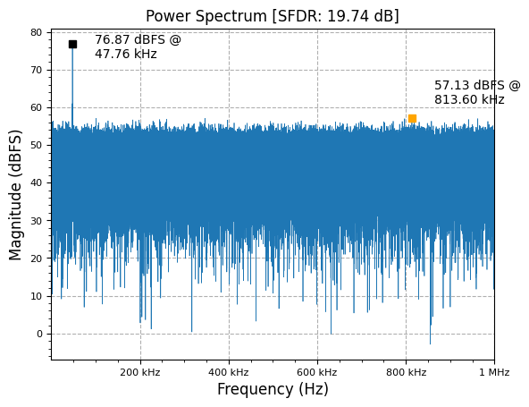
plot.spec_an(y, fs, title="Power Spectrum")

(<Figure size 640x480 with 1 Axes>, <Axes: title={'center': 'Power Spectrum [SFDR: 19.08 dB]'}, xlabel='Frequency (Hz)', ylabel='Magnitude (dBFS)'>)

png

References

Introduction to Radar Using Python and MATLAB