Cascaded Integrator–Comb (CIC) Filter

Est. read time: 3 minutes | Last updated: August 29, 2024 by John Gentile

Contents

Integrator Section
Comb Section
Bit Growth
Discrete-Time Test of CIC
References

import numpy as np
import matplotlib.pyplot as plt

from rfproto import measurements, multirate, plot, sig_gen

Benefits:

Multiplier-free implementation for economical (light resource utilization) design in digital HW systems which can handle arbitrary, and large, rate changes.
High interpolation CIC filters can push very narrowband signals (e.x. TT&C ~2MS/s max) go to sufficient ADC/DAC sample rates (e.x. 125MS/s)
Data reduction to not have to pass as much data to/from the front end (e.g. having to push full sample bandwidth data to/from a remote radio head)

CIC filters can be used as decimation (decrease sample rate) and interpolation (increase sample rate) multirate filters:

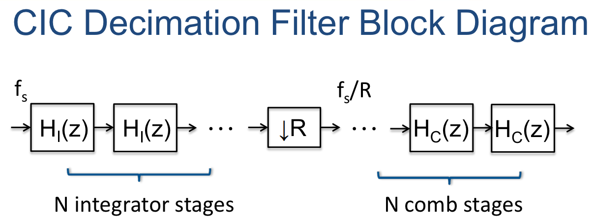
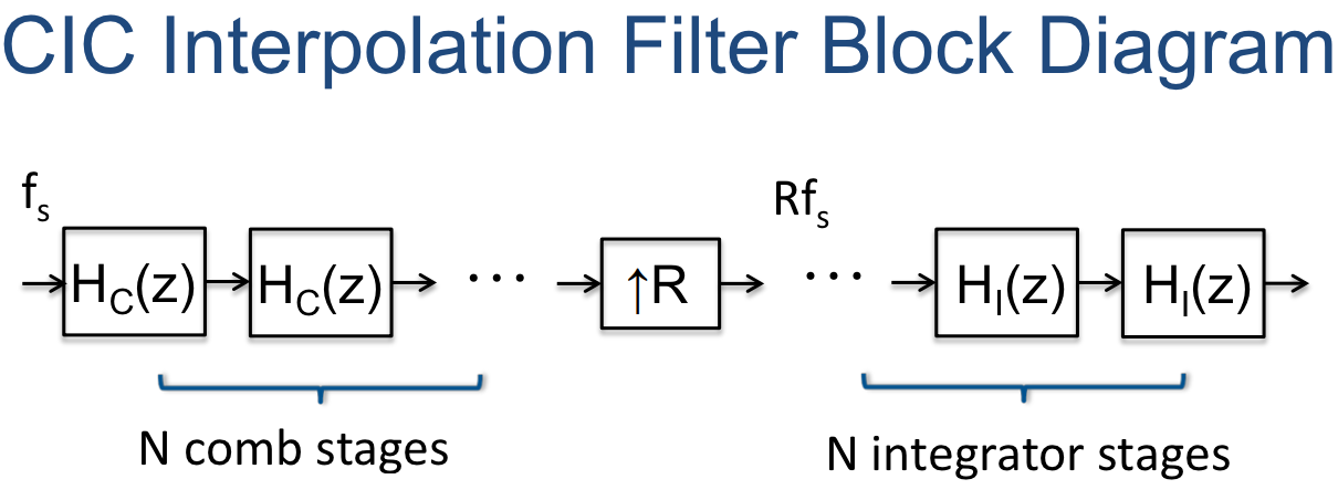
The basic building blocks are $N$ integrator and $N$ comb sections (hence the name), along with an interpolator (e.g. zero-stuffing expander) or decimator, increasing or decreasing the output sample rate by $R$ times (respectively).

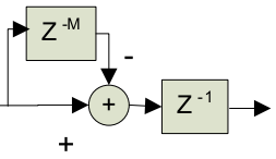
Integrator Section

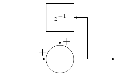
An integrator is simply a single-pole IIR filter with unity feedback coefficient:

y[n] = y[n-1] + x[n]

This is also commonly known as an accumulator, which has the $z$ -transform transfer function of:

H_{I}(z)=\frac{1}{1 - z^{-1}}

The power response is basically a low-pass filter with a −20 dB per decade (−6 dB per octave) rolloff, but with infinite gain at DC. This is due to the single pole at z = 1; the output can grow without bound for a bounded input. In other words, a single integrator by itself is unstable. - CIC Filter Introduction - Matthew P. Donadio (DSP Guru)

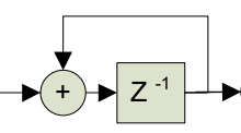
Note the pipelined version of the integrator which allows for more efficient digital hardware implementation (only one added between register stages):

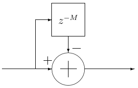
Comb Section

The comb filter runs at the highest sample rate, $f_{C} = R*f_{I}$ , in either decimation or interpolation filter form. It looks opposite of an integrator section as it subtracts the current sample value from a value $M$ sample periods prior; $M$ is the differential delay design parameter, and is often limited to $M = 1$ or $M = 2$ :

y[n] = x[n] - x[n - RM]

The corresponding transfer function at $f_{s}$ is:

H_{C}(z) = 1 - z^{-RM}

When $R=1$ and $M=1$ , the power response is a high-pass function with 20dB per decade gain (inverse of the integrator response). When $RM \neq 1$ , the power response looks like a familiar raised cosince form with $RM$ cycles from $0 \rightarrow 2\pi$ .

Bit Growth

Due to the cascaded adders/subtracters in the CIC filter, each fixed-point, two’s complement arithmetic operation requires an additional bit of output than input, to prevent loss of precision. Given an input sample bitwidth of $B_{in}$ , the output bitwidth required can be found to be:

B_{out} = \lceil N\log_{2}RM + B_{in} \rceil

At the expense of added quantization noise, bit growth can be controlled by rounding/scaling at some points within the CIC stages.

#TODO:

Look at the fred harris paper on multiplier-less CIC with sharpening that doesn’t need compensation FIR
- Also mentioned in https://www.dsprelated.com/showarticle/1337.php
For bit growth, look at CIC filter register pruning
- Also shown in http://www.jks.com/cic/cic.html and https://github.com/jks-prv/cic_prune

Discrete-Time Test of CIC

f_start = 0
f_end = 5e3
fs = 100e3
num_samples = 100000
bit_width = 16

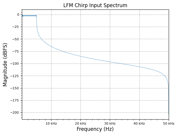
lfm_chirp_sig = np.real(sig_gen.cmplx_dt_lfm_chirp(2**(bit_width-5), f_start, f_end, fs, num_samples))
freq, y_PSD = measurements.PSD(lfm_chirp_sig, fs, real=True, norm=True)
plot.freq_sig(freq, y_PSD, "LFM Chirp Input Spectrum", scale_noise=False)
plt.show()

png

N = 3 # number of stages
R = 8 # interp/decim factor
M = 1 # differential delay in comb stages

cic_bit_width = 21 # np.ceil(N * np.log2(R*M) + bit_width)

integ_stages = [multirate.integrator(cic_bit_width) for i in range(N)]
comb_stages = [multirate.comb(M) for i in range(N)]

integ_out = np.zeros(len(lfm_chirp_sig))
for i in range(len(integ_out)):
    temp_val = int(lfm_chirp_sig[i])
    for j in range(N):
        temp_val = integ_stages[j].step(temp_val)
    integ_out[i] = temp_val

decimate_out = multirate.decimate(integ_out, R)

cic_out = np.zeros(len(decimate_out))
for i in range(len(cic_out)):
    temp_val = decimate_out[i]
    for j in range(N):
        temp_val = comb_stages[j].step(temp_val)
    cic_out[i] = temp_val

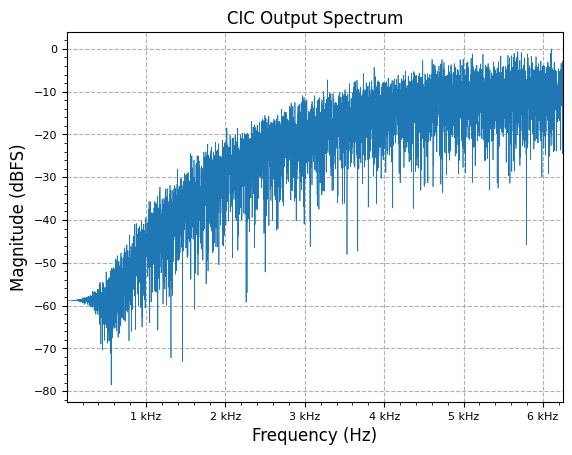
freq, y_PSD = measurements.PSD(cic_out, fs / R, real=True, norm=True)
plot.freq_sig(freq, y_PSD, "CIC Output Spectrum", scale_noise=False)
plt.show()

png

Cascaded Integrator–Comb (CIC) Filter

Integrator Section

Comb Section

Bit Growth

Discrete-Time Test of CIC

References